ipumsr - Integrating IPUMS Data with R
We are excited to announce the ipumsr R package, which helps make importing IPUMS data into R easy. Though several approaches already exist, bringing data to R hasn’t been as easy as other statistical software. We hope you’ll find that ipumsr changes this.
As a teaser, here’s just one of the many cool things you can create with IPUMS data and R.
Click on this image to launch the interactive version in a new tab.
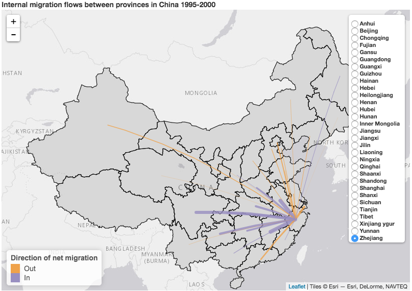
Data from China’s 2000 Census Data from IPUMS International, small numbers suppressed to maintain confidentiality. Map made with the ipumsr package and several other R packages, see the ipumsr gist on rpubs for the code and the MIGCN variable page for more details about the definition.
Setup
Unlike the syntax files available for other statistical packages, you will need to install a software package before you can import the data, using this command:
install.packages("ipumsr")
Data Import
ipumsr currently supports IPUMS microdata projects and IPUMS NHGIS. IPUMS microdata projects can be loaded using the fixed-width or csv formats combined with the DDI .xml file. You can download these files from your extract page, by right clicking the link and selecting “Save”.
Then, from R, you can load the ddi and data by running the following commands:
library(ipumsr)

# There's a small extract file from IPUMS CPS included with the package
cps_ddi <- read_ipums_ddi(ipums_example("cps_00015.xml"))
cps_data <- read_ipums_micro(cps_ddi, data_file = ipums_example("cps_00015.dat.gz"), verbose = FALSE)

head(cps_data)
#> # A tibble: 6 x 13
#>    YEAR SERIAL HWTSUPP  STATEFIP  ASECFLAG     MONTH PERNUM  WTSUPP
#>   <dbl>  <dbl>   <dbl> <int+lbl> <int+lbl> <int+lbl>  <dbl>   <dbl>
#> 1  2016  24138 3249.07        55         1         3      1 3249.07
#> 2  2016  24139 3154.25        55         1         3      1 3154.25
#> 3  2016  24139 3154.25        55         1         3      2 3154.25
#> 4  2016  24140 1652.37        55         1         3      1 1652.37
#> 5  2016  24140 1652.37        55         1         3      2 1502.68
#> 6  2016  24140 1652.37        55         1         3      3 1652.37
#> # ... with 5 more variables: AGE <int+lbl>, EDUC <int+lbl>,
#> #   INCTOT <dbl+lbl>, HEALTH <int+lbl>, MIGRATE1 <int+lbl>
If you prefer to write fewer lines of code, you can pass the ddi file directly into the read_ipums_micro() function to skip a step, but not all metadata features work without access to the DDI.
For IPUMS NHGIS data, data can be read directly out of the zipped extract file.
# And also a small NHGIS extract file in the examples
nhgis_cb <- read_ipums_codebook(ipums_example("nhgis0008_csv.zip"))
nhgis_data <- read_nhgis(ipums_example("nhgis0008_csv.zip"), verbose = FALSE)

head(nhgis_data)
#> # A tibble: 6 x 17
#>   GISJOIN  YEAR DIVISIONA MSA_CMSAA                             PMSA PMSAA
#>     <chr> <int>     <chr>     <int>                            <chr> <chr>
#> 1   G1120  1990      <NA>      1122                  Boston, MA PMSA  1120
#> 2   G1200  1990      <NA>      1122                Brockton, MA PMSA  1200
#> 3   G4160  1990      <NA>      1122 Lawrence--Haverhill, MA--NH PMSA  4160
#> 4   G4560  1990      <NA>      1122              Lowell, MA--NH PMSA  4560
#> 5   G5350  1990      <NA>      1122                  Nashua, NH PMSA  5350
#> 6   G7090  1990      <NA>      1122       Salem--Gloucester, MA PMSA  7090
#> # ... with 11 more variables: REGIONA <chr>, STATEA <chr>, ANPSADPI <chr>,
#> #   D6Z001 <int>, D6Z002 <int>, D6Z003 <int>, D6Z004 <int>, D6Z005 <int>,
#> #   D6Z006 <int>, D6Z007 <int>, D6Z008 <int>
Exploring Metadata
The ipumsr packages provides helper functions to remind yourself about the variables in your extract. You can find the variable label, variable description and value labels:
# Works for microdata projects
ipums_var_label(cps_data$WTSUPP)
#> [1] "Supplement Weight"
ipums_var_desc(cps_data$YEAR)
#> [1] "YEAR reports the year in which the survey was conducted.  YEARP is repeated on person records."
ipums_val_labels(cps_data$HEALTH)
#> # A tibble: 5 x 2
#>     val       lbl
#>   <dbl>     <chr>
#> 1     1 Excellent
#> 2     2 Very good
#> 3     3      Good
#> 4     4      Fair
#> 5     5      Poor

# And NHGIS
ipums_var_desc(nhgis_data$D6Z001)
#> [1] "Year Structure Built (D6Z)"
ipums_var_label(nhgis_data$D6Z001)
#> [1] "1989 to March 1990"
The DDI contains some additional metadata about your extract as a whole. You can find your extract notes (using ipums_file_info(cps_ddi, "extract_notes") or remind yourself of the citation you should use using ipums_file_info(cps_ddi, "citation"). For some projects and variables, you can also get a link to the original variable’s page on our website using the command ipums_website(cps_ddi, "HEALTH").
Finally, use the command ipums_view(cps_ddi) to build an interactive document based on your DDI that you can refer to:
ipums_view(cps_ddi)
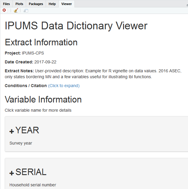 Screenshot of ipums_view in Rstudio viewer
Using Value labels
Many variables in IPUMS microdata projects contain value labels that attach a label to particular numeric values in the data (for example 1 = “No”, 2 = “Yes” and 99 = “NIU”). Because R’s factor variables do not support all of the meaning behind the way IPUMS uses these value labels, the ipumsr package uses the “labelled” class instead.
Because this is not a standard R data structure, the ipumsr package provides helper functions for translating variables to factors or numeric values.
# HEALTH is an example of a variable we can directly translate to a factor
table(cps_data$HEALTH)
#>
#>    1    2    3    4    5
#> 3559 3709 2640  746  229
table(as_factor(cps_data$HEALTH))
#>
#> Excellent Very good      Good      Fair      Poor
#>      3559      3709      2640       746       229

# In INCTOT the labelled values actually refer to missings - the function lbl_na_if() is helpful
# Note that lbl_na_if can refer to the variable's values by value or label
range(cps_data$INCTOT)
#> [1]   -10399 99999999
range(lbl_na_if(cps_data$INCTOT, ~.val > 90000000), na.rm = TRUE)
#> [1]  -10399 1230006
range(lbl_na_if(cps_data$INCTOT, ~.lbl %in% c("Missing.", "N.I.U. (Not in Universe).")), na.rm = TRUE)
#> [1]  -10399 1230006

# In EDUC, IPUMS CPS includes a hierarchical label system. The function lbl_collapse can help use
# the less detailed version
head(table(as_factor(
  cps_data$EDUC
)))
#>
#>  NIU or no schooling         NIU or blank    None or preschool
#>                    0                 2689                   17
#> Grades 1, 2, 3, or 4              Grade 1              Grade 2
#>                   18                    0                    0

head(table(as_factor(
  lbl_collapse(cps_data$EDUC, ~.val %/% 10)
)))
#>
#>  NIU or no schooling Grades 1, 2, 3, or 4        Grades 5 or 6
#>                 2706                   18                   47
#>        Grades 7 or 8              Grade 9             Grade 10
#>                  232                  223                  267
See the ‘value-labels’ vignette included with the package for more details.
Using Geographic Metadata
IPUMS NHGIS and some microdata project provide geographic boundary files that correspond to your extract. For IPUMS NHGIS data, the boundary files are provided alongside your extract and ipumsr provides a single function to load both the data and the boundaries.
nhgis <- read_nhgis_sf(
  ipums_example("nhgis0008_csv.zip"),
  shape_file = ipums_example("nhgis0008_shape_small.zip"),
  verbose = FALSE
)

nhgis$`Percent of Homes Built Before 1950, by PMSA` <- with(
  nhgis,
  (D6Z007 + D6Z008) / (D6Z001 + D6Z002 + D6Z003 + D6Z004 + D6Z005 + D6Z006 + D6Z007 + D6Z008)
)

# sf has some basic built-in plotting capababilities (ggplot2 support coming in the next version)
plot(nhgis[, c("Percent of Homes Built Before 1950, by PMSA", "geometry")])
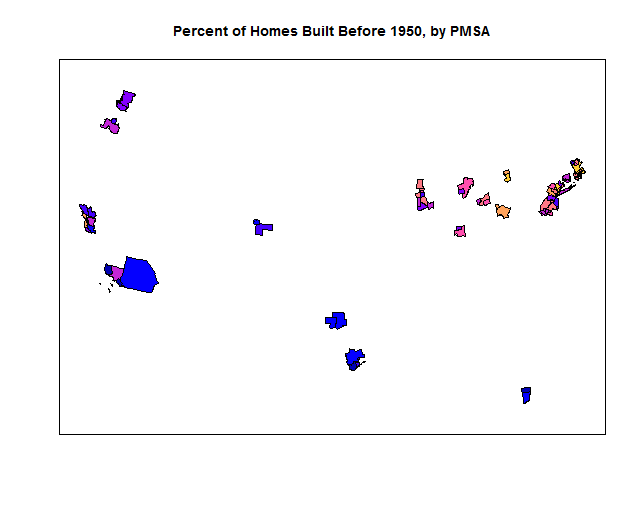 Percent of Homes Built Before 1950, by PMSA
Several IPUMS microdata projects also provide geographic data, which can be loaded with the function read_ipums_sf().
Tap into R’s powerful ecosystem
And with that, your IPUMS data is available to you in R! If you’re new to R or want to learn more about it, there’s a lot of great resources. Some that we know of are:
- DataCamp’s free introduction to R course
- R for Data Science by Garret Rolemund and Hadley Wickham
- The John Hopkins MOOC R Programming
Technical Challenges
Here I describe some of the design challenges of loading IPUMS data into R and how we solved them.
Value labels don’t fit in factors
A valuable part of IPUMS harmonization process is that we add meaningful and consistent value labels to our data. At first glance, base R’s often maligned and misunderstood data structure factors seems like a natural fit. However, factors are incompatible with the way IPUMS (and other statistical software) treat labelled values in two ways:
-
The numeric value of a factor must be a sequence. Many IPUMS variables have value labels that indicate missing/unusual values with large numbers to set them apart from the rest of the values. Factors on the other hand are always structure so that the first label gets the value 1, the second 2, etc.
-
All values in a factor must be labelled. In IPUMS data, for variables like AGE and INCOME, most of the values are unlabelled, but we add special values for things like NIU (not in universe), Unknown, Missing Responses, etc. But in base R, all values in a factor must have a label.
The ipumsr package is not the first time R developers have encountered this problem, so we were able to build off the existing approach in the haven package. ipumsr imports the labels into haven’s labelled objects, and then provides helper functions like lbl_collapse(), lbl_na_if() and lbl_clean() that are designed to make it easier to work with the conventions most IPUMS labels follow. See the labelled values vignette for more details.
Base R’s read.fwf/read.csv are slow
Functions like readr::read_fwf for fixed width files and readr::read_csv or data.table::fread (among others) are much faster than the base R functions like read.csv and read.fwf. In my tests, readr::read_fwf is about 40 times faster than read.fwf. To make matters worse, IPUMS hierarchical data have widths that change depending on the record type, which none of these functions support. The ipumsr package uses readr functions when possible, but has C++ code to handle the hierarchical files. Winston Chang’s package profvis provides a wonderful interface for making flame graphs in R, so it was easy to find the performance bottlenecks.
Using other IPUMS metadata
We also wanted to make the IPUMS metadata like the value labels, variable labels, variable descriptions and geographic boundary files as easy to use as possible. Beyond the labelled values helpers mentioned above, you can peruse the value labels and variable descriptions interactively using ipums_view(), read and merge geographic data from IPUMS using read_ipums_shape() and ipums_shape_left_join(), and hopefully more coming soon.
We’d love your feedback on ipumsr, either by email to ipums@umn.edu or on github!
Authored by Greg Freedman Ellis
Code
R