Modern Contraceptive Method Mix is a core indicator in the FP2030 Measurement Framework representing the distribution of modern method users by method. Researchers use this distribution to understand which family planning methods are preferred and accessible in a particular place.

While there is no “right” method mix or “ideal” method, there is general agreement that providing access to a wide variety of methods is both a component of quality of care as well as an important principle of rights-based family planning.

— FP2030 Core Indicators

Modern Method Mix can change year-to-year in response to the introduction of new methods in-country, access restrictions (e.g. stockouts), increased need for specific methods (e.g. those that protect against sexually transmitted infections), and shifting user preferences.¹ Cross-sectional PMA surveys are fielded approximately once per year, allowing researchers to monitor these changes at annual intervals. Typically, you’ll find “Trends in Modern Contraceptive Mix” updated in the PMA Survey Results Summary published for each new sample.

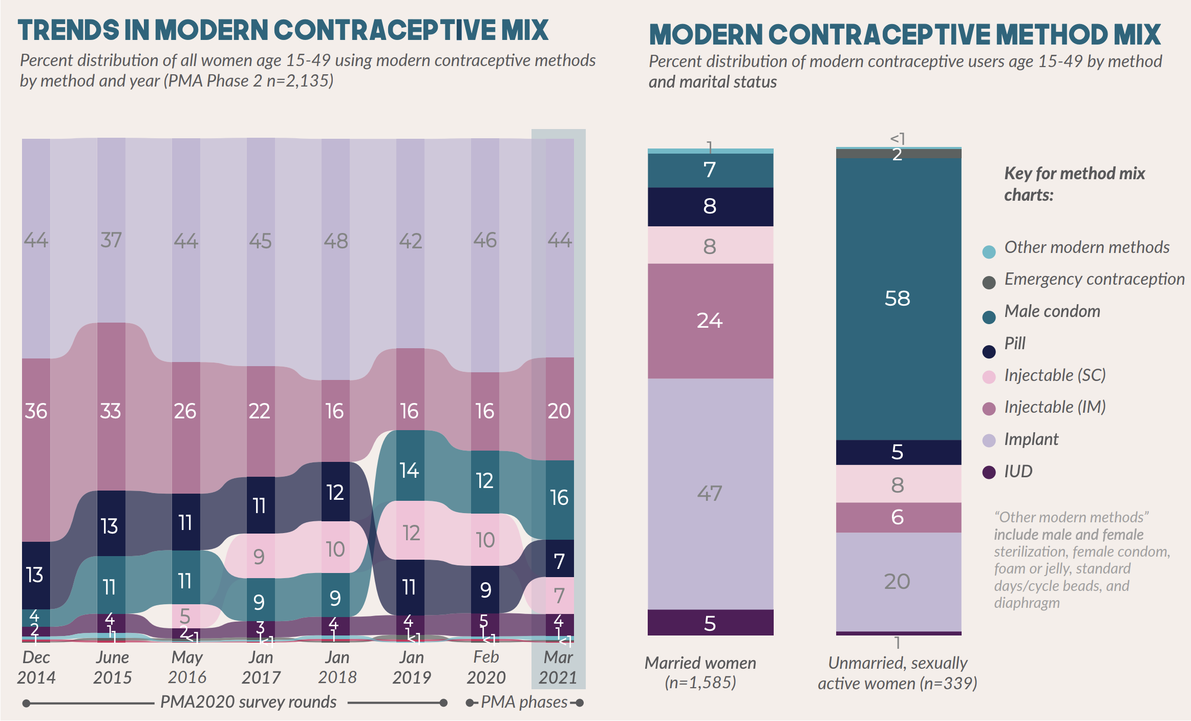
In this post, we’ll show how you can make a graphic similar to this one in R using a single data extract downloaded from IPUMS PMA. We’ll be focusing on Modern Method Mix, but we recommend using IPUMS data any time you want to investigate how indicators change over time or how they compare across populations. That’s because the IPUMS PMA data extract system is designed both to allow researchers to combine data from multiple samples and to flag important comparability issues between those samples.

Setup

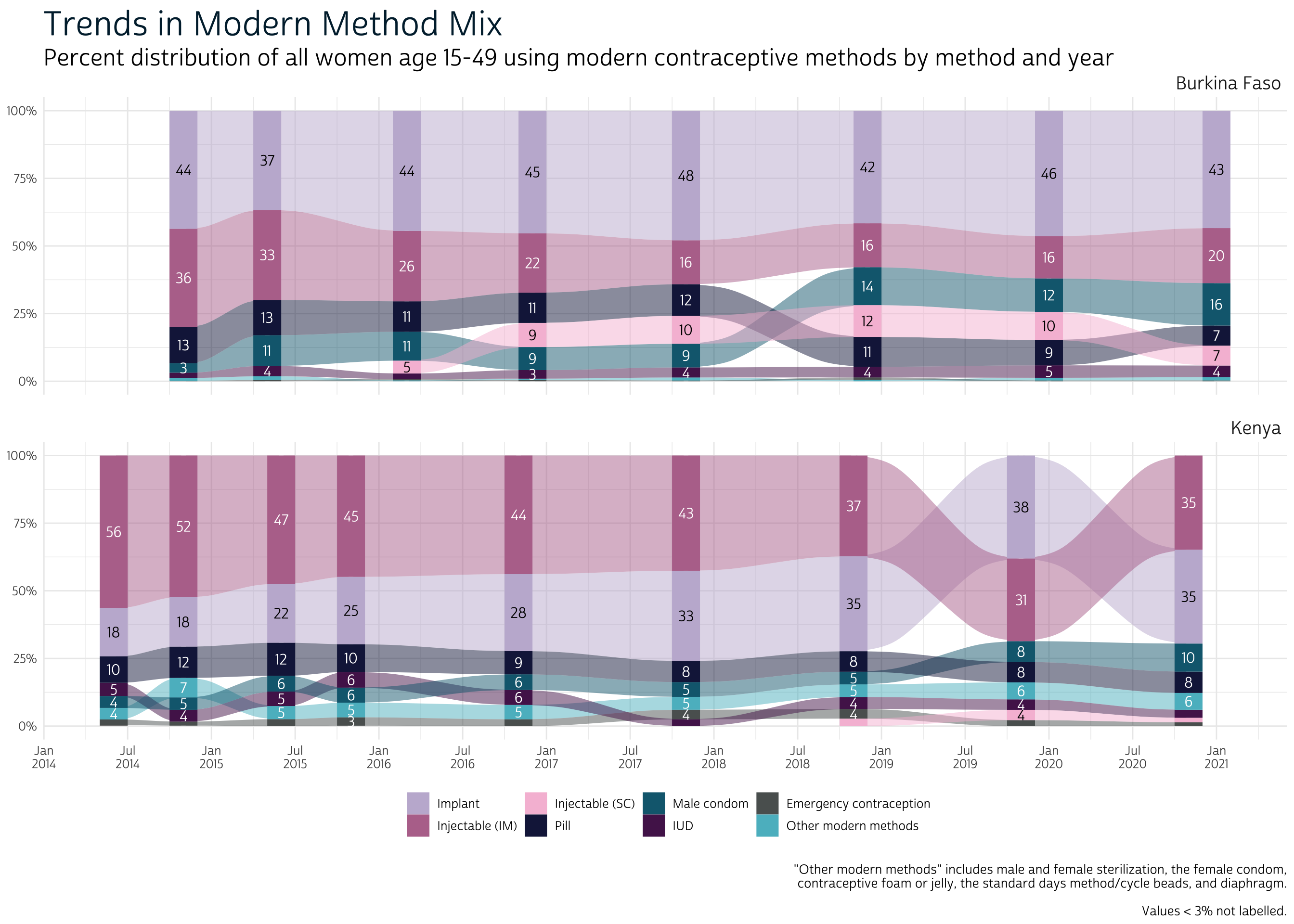
You can compare trends in Modern Method Mix for any number of PMA samples with a single data extract from IPUMS PMA. Here, we’ll illustrate using data from two countries, Burkina Faso and Kenya, where cross-sectional data have been collected continuously between 2014 and 2021.

Country	Sample Year	Data Collection Period
Burkina Faso	2014	Nov 2014 - Jan 2015
	2015	Apr 2015 - June 2015
	2016a	Mar 2016 - Apr 2016
	2016b	Nov 2016 - Feb 2017
	2017	Nov 2017 - Jan 2018
	2018	Dec 2018 - Jan 2019
	2020	Dec 2019 - Feb 2020
	2021	Dec 2020 - Mar 2021
Kenya	2014a	May 2014 - Aug 2014
	2014b	Nov 2014 - Dec 2014
	2015a	Jun 2015 - Jul 2015
	2015b	Nov 2015 - Dec 2015
	2016	Nov 2016 - Dec 2016
	2017	Nov 2017 - Dec 2017
	2018	Nov 2018 - Jan 2019
	2019	Nov 2019 - Dec 2019
	2020	Nov 2020 - Dec 2020

Our extract will contain all of these cross-sectional samples, filtered to include only Female Respondents. It will also contain the following variables:

We’ll load the extract and a few key packages into R like so:

# Load packages 
library(ipumsr)
library(tidyverse)
library(srvyr)
library(ggalluvial)

# Load data extract 
dat <- read_ipums_micro(
  ddi = "data/pma_00165.xml",
  data = "data/pma_00165.dat.gz"
)

Additionally, we’ll modify a few variables to improve readability:

A Century Month Code (CMC) we call INTFQCMC will be created for each individual woman’s interview date²
We’ll store the median interview date for each sample in INTFQMED
All key categorical variables will be recoded with as_factor

dat <- dat %>% 
  group_by(SAMPLE) %>% 
  mutate(
    INTFQCMC = 12*(INTFQYEAR - 1900) + INTFQMON,
    INTFQMED = median(INTFQCMC), 
    across(
      c(COUNTRY, INTFQMON, TIMEMENSTRUATE, MCP, FPCURRUSE, FPCURREFFMETH,
        FPCURREFFMETHRC, FPEFFECTIVEYR, FPCURRINJTYPE, FP1STMETHOD, MARSTAT),
      as_factor
    )
  ) %>% 
  ungroup()

Most Effective Method

PMA surveys ask each woman to report all family planning methods she or her partner are currently using to delay or avoid getting pregnant. The question looks something like this one, where the respondent is prompted to select all options that apply:

Which method or methods are you using?

PROBE: Anything else?

Select all methods mentioned. 
SCROLL TO THE BOTTOM to see all choices.

  [] Female sterilization
  [] Male sterilization
  [] Implant
  [] IUD
  [] Injectables
  [] Pill
  [] Emergency Contraception
  [] Male condom
  [] Female condom
  [] Diaphragm
  [] Foam/Jelly
  [] Standard Days/Cycle beads
  [] LAM
  [] Rhythm method
  [] Withdrawal
  [] Other traditional method
  [] No response

Because a woman can report more than one method, PMA ranks the effectiveness of each method and uses only her most effective method to calculate Modern Method Mix. This ensures that sum of all methods included in Modern Method Mix is 100%.

Every PMA sample includes a variable FPCURREFFMETH that indicates the most effective method reported by the respondent on this question. However, it’s important to note that the list of methods may vary between samples.

Fortunately, IPUMS makes it easy to identify whether each method is available for the researcher’s samples of interest. On the FPCURREFFMETH codes tab, we see the availability of every method in each sample from Burkina Faso and Kenya.

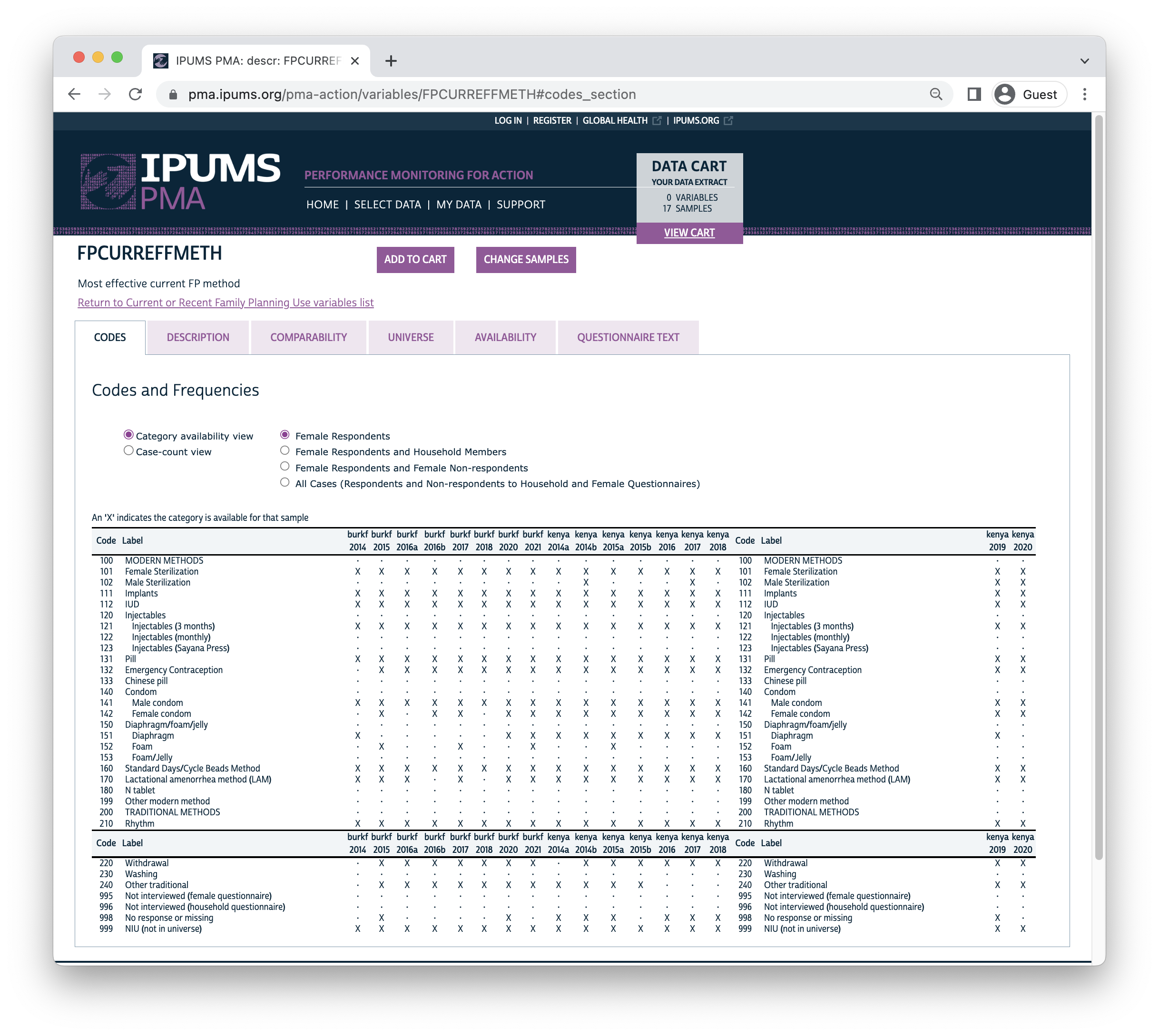
Certain methods like N-tablet, Washing, or “Other Modern” were included in none of our samples. Others, like Diaphragm and Foam, appear intermittently: these methods may have been listed on the questionnaire, but appear unavailable if no women selected the associated response option (or if they were only selected in combination with a more effective method).

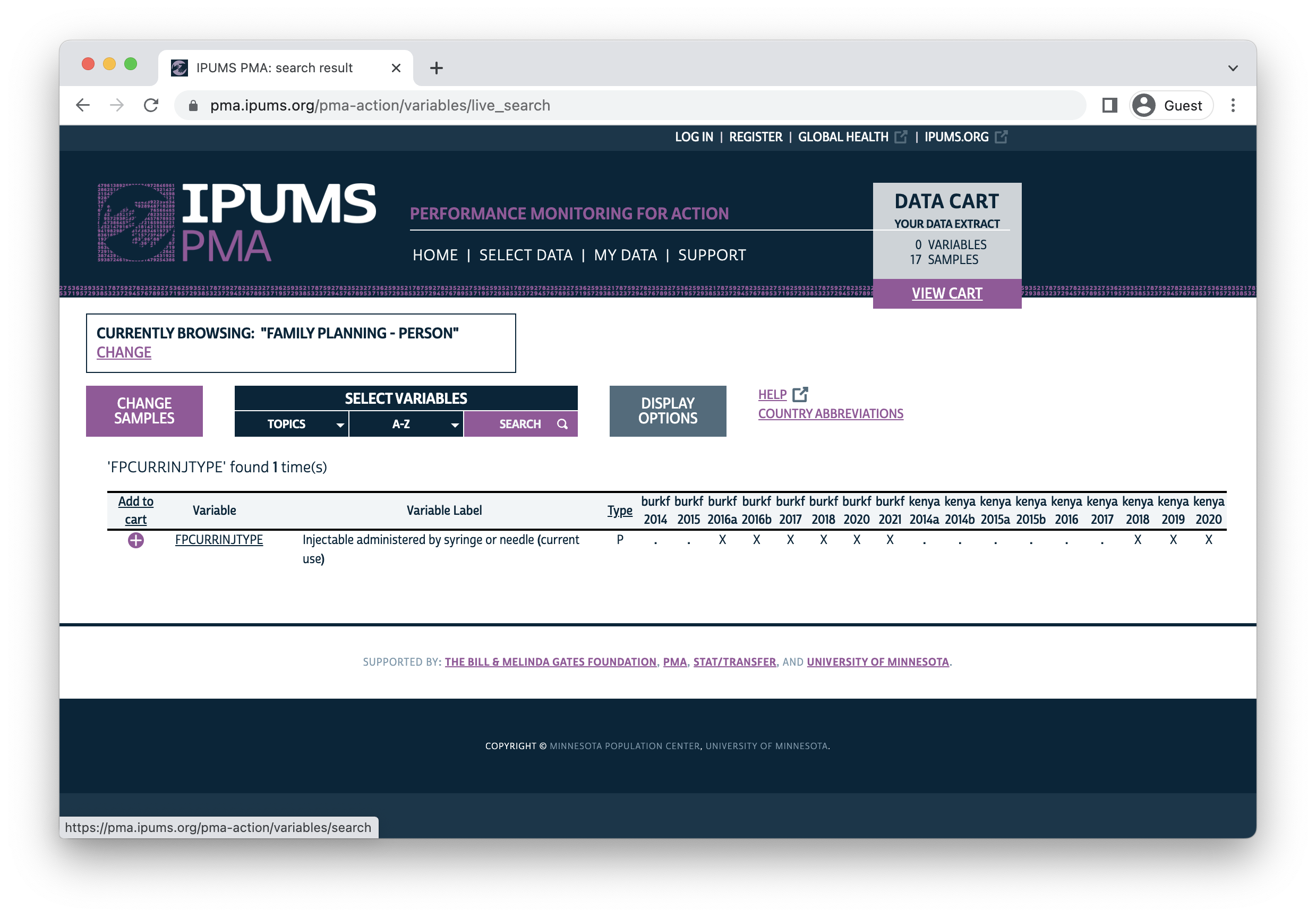
FPCURREFFMETH uses composite coding, where general categories like Injectables (code 120) are used if a particular questionnaire did not distinguish between specific sub-categories like 3-month, monthly, or Sayana Press (codes 121, 122, and 123). In Burkina Faso and Kenya samples, women were not asked to specify injectable type on this question; however, later samples included the following supplementary question (accompanied by a visual aid):

Was the injection administered via syringe or small needle?

Show the image to the respondent.

  [] Syringe
  [] Small needle (Sayana Press)
  [] No response

Responses to this question are recorded in the variable FPCURRINJTYPE. The IPUMS system shows that it was added to Burkina Faso samples beginning in 2016, and that it was added to Kenya samples beginning in 2018:

Recoding

When the supplementary question associated with FPCURRINJTYPE was added, PMA released a recoded version of most effective method that you’ll find in FPCURREFFMETHRC (the suffix RC indicates “recoded”). This variable makes four adjustments to the original variable FPCURREFFMETH (see description tab):

Women who report Sayana Press in FPCURRINJTYPE are differentiated from those using 3-month injectables. (Sayana Press users are identified as “Injectable (SC)” in the graphic at the top of this post.)
Women who report using the lactational amenorrhea method (LAM) in FPCURREFFMETH are coded “other traditional” in FPCURREFFMETHRC if they fail to meet the criteria for effective use of LAM. Specifically, LAM users must be less than six months post-partum (see LASTDOBCMC) and amenorrheic / not currently menstruating (see TIMEMENSTRUATE and TIMEMENSTRUATEVAL).
Women who did not report current use of a contraceptive method (coded “NIU (not in universe)” in FPCURREFFMETH) are coded “emergency contraception” in FPCURREFFMETHRC if they reported using an emergency method at all in the last 12 months (see FPEFFECTIVEYR, or FPECUSYR for later samples).
Women who did not report using Female Sterilization as a current method in FPCURREFFMETH are coded “female sterilization” if they indicated elsewhere that they had been sterilized (see FP1STMETHOD).

PMA uses FPCURREFFMETHRC in its calculation of Modern Method Mix, but FPCURREFFMETHRC was not retroactively added to older samples. We’ll demonstrate how to recode FPCURREFFMETH manually for samples where FPCURREFFMETHRC is not available.

Notably, we won’t be able to identify users of Sayana Press for samples prior to the introduction of FPCURRINJTYPE (this explains the apparent growth from 0% in June 2015 to 5% in May 2016 in the Burkina Faso graphic at the top of this post).

Instead, we’ll begin with the adjustment made for LAM users who are not post-partum amenorrheic (PPA). Unfortunately, PMA does not include a variable indicating whether women are PPA, so we’ll need to make our own variable called PPA.

# `TIMEMENSTRUATE` gives a unit, while `TIMEMENSTRUATEVAL` gives a value
# We use these variables to calculate months since last period: `MENSTR_MOS`
dat <- dat %>% 
  mutate(
    MENSTR_MOS = case_when(
      TIMEMENSTRUATE == "Days" ~ TIMEMENSTRUATEVAL / 30,
      TIMEMENSTRUATE == "Weeks" ~ TIMEMENSTRUATEVAL / 4,
      TIMEMENSTRUATE == "Months" ~ TIMEMENSTRUATEVAL %>% as.double,
      TIMEMENSTRUATE == "Years" ~ TIMEMENSTRUATEVAL * 12
    ) 
  )

# `INTFQCMC` gives the month of the interview, while
# `LASTDOBCMC` gives the month of most recent birth (or 9999 for no prior birth) 
# The difference is the number of months since last birth: `BIRTH_MOS`
dat <- dat %>% 
  mutate(
    BIRTH_MOS = case_when(
      LASTDOBCMC < 9000 ~ INTFQCMC - LASTDOBCMC
    ) 
  )

# `TIMEMENSTRUATE` can also be "Before last birth" 
# If so, or if MENSTR_MOS > BIRTH_MOS, women who gave birth < 6 months are PPA
# All others are not PPA (or NA if most recent period cannot be determined)
dat <- dat %>% 
  mutate(
    PPA = case_when(
      BIRTH_MOS < 6 & TIMEMENSTRUATE == "Before last birth" ~ TRUE,
      BIRTH_MOS < 6 & MENSTR_MOS > BIRTH_MOS ~ TRUE,
      BIRTH_MOS >= 6 | LASTDOBCMC > 9000 ~ FALSE
    )
  )

We use our PPA variable together with FP1STMETHOD and FPEFFECTIVEYR to manually build FPCURREFFMETHRC for early samples where it is not available. Otherwise, we use the version of FPCURREFFMETHRC provided by PMA for later samples.

dat <- dat %>% 
  mutate(
    FPCURREFFMETHRC = case_when(
      !is.na(`FPCURREFFMETHRC`) ~ FPCURREFFMETHRC %>% as_factor %>% as.character,
      FP1STMETHOD == "Female sterilization" ~ "Female Sterilization",
      FPCURRUSE != "Yes" & FPEFFECTIVEYR == "Emergency Contraception" ~ "Emergency Contraception",
      FPCURREFFMETH == "Lactational amenorrhea method (LAM)" & !PPA ~ "Other traditional",
      TRUE ~ FPCURREFFMETH %>% as_factor %>% as.character
    )
  )

You can review the changes made to FPCURREFFMETH in FPCURREFFMETHRC like so:

dat %>% 
  filter(FPCURREFFMETH != FPCURREFFMETHRC) %>% 
  count(FPCURREFFMETH, FPCURREFFMETHRC)

# A tibble: 7 × 3
  FPCURREFFMETH                       FPCURREFFMETHRC                n
  <fct>                               <chr>                      <int>
1 IUD                                 Female Sterilization           1
2 Injectables (3 months)              Female Sterilization           1
3 Injectables (3 months)              Injectables (Sayana Press)   895
4 Female condom                       Female Sterilization           1
5 Lactational amenorrhea method (LAM) Other traditional            108
6 NIU (not in universe)               Emergency Contraception      314
7 NIU (not in universe)               Female Sterilization           7

Modern Method Users

When we calculate Modern Method Mix, we’ll determine the share of women who use each method as a proportion of women age 15-49 who use any modern method. Every PMA sample includes a variable MCP indicating whether the woman is currently using a modern method (any method except Rhythm, Withdrawal, or Other Traditional).

MCP also uses the woman’s most effective current method if she indicates that she is using more than one method. Fortunately, MCP uses the same recoding logic shown for FPCURREFFMETHRC above: it adjusts for non-PPA use of LAM, Emergency Contraception within the past year, and prior sterilization (see description tab for details). Because MCP is available for every PMA sample, we need to make no additional changes here.

Missing values

MCP includes the values “Yes”, “No”, and “No response or missing”. If you compare MCP with FPCURREFFMETH, you’ll see that there are several cases where MCP is “missing” even though the woman reported use of a method:

dat %>% 
  filter(MCP == "No response or missing") %>% 
  count(MCP, FPCURREFFMETH)

# A tibble: 14 × 3
   MCP                    FPCURREFFMETH                           n
   <fct>                  <fct>                               <int>
 1 No response or missing Female Sterilization                    3
 2 No response or missing Implants                              149
 3 No response or missing IUD                                    20
 4 No response or missing Injectables (3 months)                 93
 5 No response or missing Pill                                   36
 6 No response or missing Emergency Contraception                 7
 7 No response or missing Male condom                            48
 8 No response or missing Female condom                           2
 9 No response or missing Standard Days/Cycle Beads Method        5
10 No response or missing Lactational amenorrhea method (LAM)     2
11 No response or missing Rhythm                                 25
12 No response or missing Withdrawal                              4
13 No response or missing Other traditional                       1
14 No response or missing NIU (not in universe)                 805

How can this be? A strong majority of these cases are women who were not members of the de facto population of women who slept in the household during the night before the household screening interview (see RESIDENT). As a result, they are not considered part of the analytic sample, and they are assigned a weight of 0 in FQWEIGHT: these cases drop out in weighted population inference (or we can drop them ourselves to suppress a warning message).

dat %>% 
  filter(MCP == "No response or missing") %>% 
  count(FQWEIGHT == 0)

# A tibble: 2 × 2
  `FQWEIGHT == 0`     n
  <lgl>           <int>
1 FALSE              35
2 TRUE             1165

The remaining 35 cases are women who were missing data on one or more of the variables used in recoding for MCP. We’ll keep them in our data in order to calculate the correct degrees of freedom for each sample.

Modern Method Mix

Finally, we’re ready to use FPCURREFFMETHRC and MCP to calculate Modern Method Mix. PMA uses a stratified cluster-sample design, so we’ll use the variables EAID and STRATA together with FQWEIGHT as survey design information.

Because our data extract contains multiple samples, we’ll need to use group_by to iterate through each independent sample (identified by our labeling variables COUNTRY and INTFQMED). To make this easier, we’ll use two nested summarise functions:

The outer summarise function allows us to specify survey design information for each independent sample (referenced iteratively as cur_data)
The inner summarise function estimates the proportion of women for each combination of MCP and FPCURREFFMETHRC in each population

dat %>% 
  filter(FQWEIGHT > 0) %>% 
  group_by(COUNTRY, INTFQMED) %>% 
  summarise(
    .groups = "keep",
    cur_data() %>% 
      as_survey_design(weights = FQWEIGHT, ids = EAID, strata = STRATA) %>% 
      group_by(MCP = as_factor(MCP), FPCURREFFMETHRC) %>% 
      summarise(survey_mean(prop = TRUE, prop_method = "logit", vartype = "ci"))
  )

# A tibble: 288 × 7
# Groups:   COUNTRY, INTFQMED [17]
   COUNTRY      INTFQMED MCP   FPCURREFFMETHRC                      coef    `_low`  `_upp`
   <fct>           <dbl> <fct> <chr>                               <dbl>     <dbl>   <dbl>
 1 Burkina Faso     1379 No    NIU (not in universe)            0.999    0.996     1.00   
 2 Burkina Faso     1379 No    Other traditional                0.000203 0.0000272 0.00151
 3 Burkina Faso     1379 No    Rhythm                           0.000672 0.0000903 0.00497
 4 Burkina Faso     1379 Yes   Diaphragm                        0.00102  0.000134  0.00765
 5 Burkina Faso     1379 Yes   Emergency Contraception          0.00163  0.000220  0.0120 
 6 Burkina Faso     1379 Yes   Female Sterilization             0.00416  0.00128   0.0135 
 7 Burkina Faso     1379 Yes   Implants                         0.436    0.358     0.518  
 8 Burkina Faso     1379 Yes   Injectables (3 months)           0.363    0.287     0.446  
 9 Burkina Faso     1379 Yes   IUD                              0.0194   0.00836   0.0445 
10 Burkina Faso     1379 Yes   Male condom                      0.0349   0.0157    0.0758 
11 Burkina Faso     1379 Yes   Pill                             0.134    0.0986    0.181  
12 Burkina Faso     1379 Yes   Standard Days/Cycle Beads Method 0.00544  0.00204   0.0144 
13 Burkina Faso     1385 No    NIU (not in universe)            0.989    0.982     0.993  
14 Burkina Faso     1385 No    No response or missing           0.000221 0.0000294 0.00166
15 Burkina Faso     1385 No    Other traditional                0.00121  0.000306  0.00478
16 Burkina Faso     1385 No    Rhythm                           0.00848  0.00514   0.0139 
17 Burkina Faso     1385 No    Withdrawal                       0.00157  0.000502  0.00493
18 Burkina Faso     1385 Yes   Emergency Contraception          0.00463  0.00172   0.0124 
19 Burkina Faso     1385 Yes   Female condom                    0.00287  0.000652  0.0126 
20 Burkina Faso     1385 Yes   Female Sterilization             0.00373  0.00123   0.0113 
# … with 268 more rows
# ℹ Use `print(n = ...)` to see more rows

Here, coef sums to 100% for each level of MCP, while the columns _low and _upp report a 95% confidence interval for each estimate. Because we’re only concerned with Modern Method Mix, we can disregard any rows where MCP != "Yes".

Data Visualization

To match the PMA graphic shown at the top of this post, we’ll make a few minor modifications to our summary table. First, we’ll combine a few of the lesser-used modern methods under “Other Modern Method”:

Male Sterilization
Female Sterilization
Female Condom
Foam
Standard Days / Cycle Beads
Diaphragm
LAM³

You can use fct_collapse to combine several factors levels into a new level like “other”. Conveniently, you can also use it to relabel levels as shown here for Implant, Injectable (IM), Injectable (SC), and Emergency contraception:

dat <- dat %>% 
  mutate(
    FPCURREFFMETHRC = FPCURREFFMETHRC %>% 
      fct_collapse(
        "Other modern methods" = c(
          "Male Sterilization", "Female Sterilization", "Female condom",
          "Foam", "Standard Days/Cycle Beads Method", "Diaphragm",
          "Lactational amenorrhea method (LAM)"
        ),
        "Implant" = "Implants",
        "Injectable (IM)" = "Injectables (3 months)",
        "Injectable (SC)" = "Injectables (Sayana Press)",
        "Emergency contraception" = "Emergency Contraception",
      ) 
  )

We’ll now save the revised summary table as a data frame called mix_tbl. We’ll also remove any of the rows that aren’t necessary to calculate Modern Method Mix (where MCP is “No” and “No response or missing”).

mix_tbl <- dat %>% 
  filter(FQWEIGHT > 0) %>% 
  group_by(COUNTRY, INTFQMED) %>% 
  summarise(
    .groups = "keep",
    cur_data() %>% 
      as_survey_design(weights = FQWEIGHT, ids = EAID, strata = STRATA) %>% 
      group_by(MCP = as_factor(MCP), FPCURREFFMETHRC) %>% 
      summarise(survey_mean(prop = TRUE, prop_method = "logit", vartype = "ci"))
  ) %>% 
  filter(MCP == "Yes")

mix_tbl

# A tibble: 131 × 7
# Groups:   COUNTRY, INTFQMED [17]
   COUNTRY      INTFQMED MCP   FPCURREFFMETHRC            coef   `_low` `_upp`
   <fct>           <dbl> <fct> <fct>                     <dbl>    <dbl>  <dbl>
 1 Burkina Faso     1379 Yes   Other modern methods    0.0106  0.00517  0.0217
 2 Burkina Faso     1379 Yes   Emergency contraception 0.00163 0.000220 0.0120
 3 Burkina Faso     1379 Yes   Implant                 0.436   0.358    0.518 
 4 Burkina Faso     1379 Yes   Injectable (IM)         0.363   0.287    0.446 
 5 Burkina Faso     1379 Yes   IUD                     0.0194  0.00836  0.0445
 6 Burkina Faso     1379 Yes   Male condom             0.0349  0.0157   0.0758
 7 Burkina Faso     1379 Yes   Pill                    0.134   0.0986   0.181 
 8 Burkina Faso     1385 Yes   Other modern methods    0.0138  0.00680  0.0278
 9 Burkina Faso     1385 Yes   Emergency contraception 0.00463 0.00172  0.0124
10 Burkina Faso     1385 Yes   Implant                 0.367   0.272    0.473 
11 Burkina Faso     1385 Yes   Injectable (IM)         0.333   0.226    0.459 
12 Burkina Faso     1385 Yes   IUD                     0.0383  0.0194   0.0742
13 Burkina Faso     1385 Yes   Male condom             0.114   0.0744   0.169 
14 Burkina Faso     1385 Yes   Pill                    0.130   0.0947   0.177 
15 Burkina Faso     1395 Yes   Other modern methods    0.00325 0.000656 0.0159
16 Burkina Faso     1395 Yes   Emergency contraception 0.00502 0.00215  0.0117
17 Burkina Faso     1395 Yes   Implant                 0.444   0.382    0.508 
18 Burkina Faso     1395 Yes   Injectable (IM)         0.261   0.194    0.341 
19 Burkina Faso     1395 Yes   Injectable (SC)         0.0477  0.0297   0.0756
20 Burkina Faso     1395 Yes   IUD                     0.0203  0.0120   0.0342
# … with 111 more rows
# ℹ Use `print(n = ...)` to see more rows

With these revisions in place, we’re now ready to make our plot. We’ve showcased the excellent ggalluvial package in earlier posts, so we won’t dig into the details too deeply here. In short: we use geom_stratum to build stacked bars for each sample, and we use geom_flow to show change over time. The argument decreasing = FALSE ensures that the methods are arranged in order of popularity for each sample.

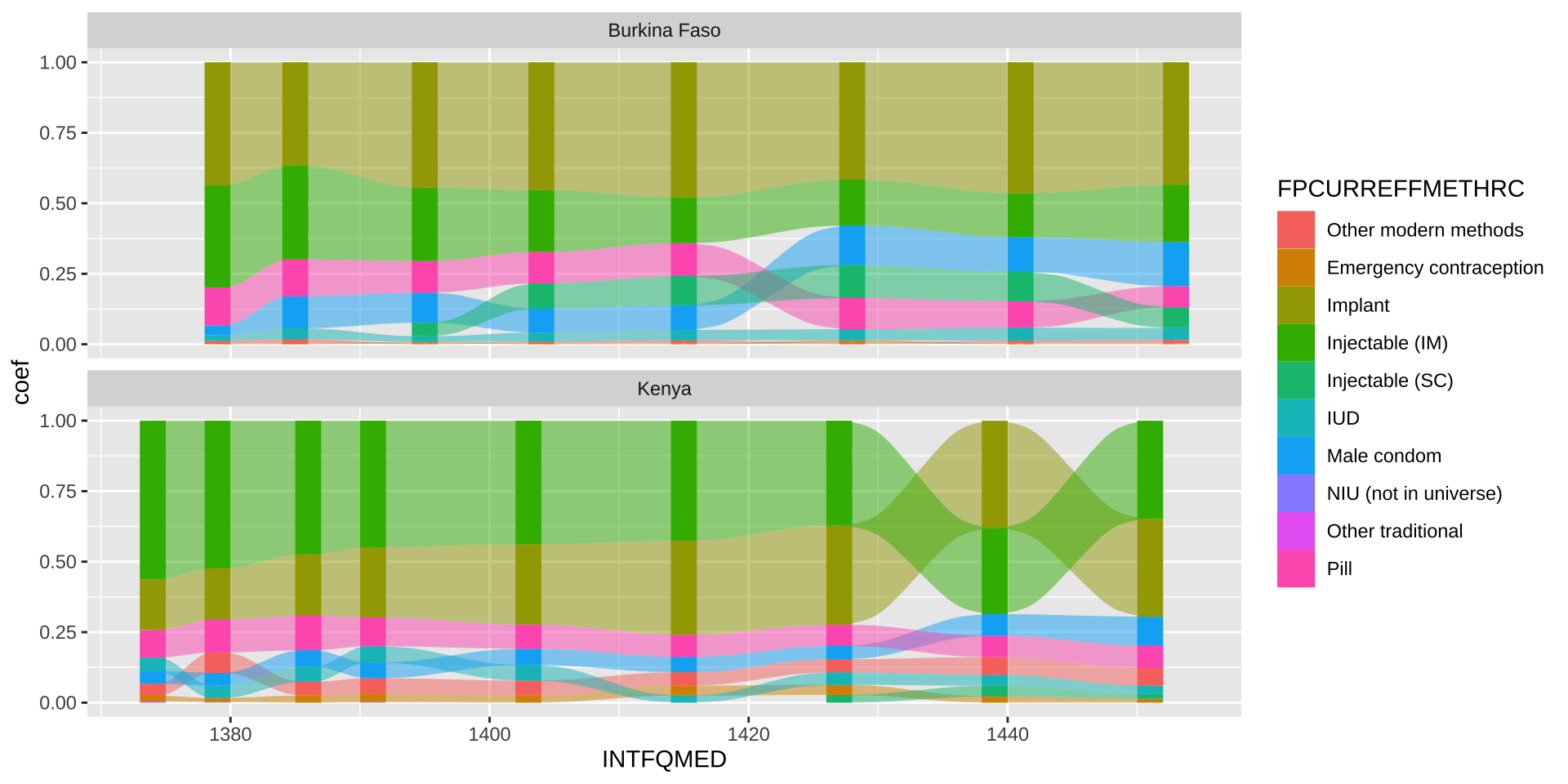
A basic alluvial plot can be made like so:

mix_plot <- mix_tbl %>% 
  ggplot(aes(
    x = INTFQMED, 
    y = coef,
    fill = FPCURREFFMETHRC,
    stratum = FPCURREFFMETHRC,
    alluvium = FPCURREFFMETHRC
  )) + 
  facet_wrap(vars(COUNTRY), ncol = 1) + 
  geom_flow(decreasing = FALSE) + 
  geom_stratum(size = 0, width = 2, decreasing = FALSE)

mix_plot

As always, we’ll apply our own custom theme and labels to clean-up the final result. If you intend to make multiple plots with the same theme, we recommend saving it as a function; we’ll call ours theme_pma.

# Fonts 
library(showtext)
sysfonts::font_add(
  family = "cabrito", 
  regular = "../../fonts/cabritosansnormregular-webfont.ttf"
)
showtext_auto()

# Fonts for geom_text
update_geom_defaults("text", list(family = "cabrito", size = 4))

# Theme 
theme_pma <- function(){
  components <- list(
    # Edit `theme_minimal`
    theme_minimal() %+replace% theme(
      text = element_text(family = "cabrito", size = 12),
      plot.title = element_text(size = 26, color = "#00263A",
                                hjust = 0, margin = margin(b = 5)),
      plot.subtitle = element_text(hjust = 0, margin = margin(b = 0), size = 18),
      plot.caption = element_text(hjust = 1, size = 10, margin = margin(t = 15)),
      plot.caption.position = "plot",
      strip.background = element_blank(),
      strip.text.x = element_text(size = 14, hjust = 1),
      strip.text.y = element_text(size = 14, angle = 0),
      panel.spacing = unit(1, "lines"),
      legend.position = "bottom",
      legend.title = element_blank()
    ) ,
    
    # Add breaks by percent to y-axis, dates to x-axis
    scale_y_continuous(labels = scales::label_percent()),
    scale_x_continuous(
      breaks = map(2014:2021, ~c(12*(.x - 1900) + 1, 12*(.x - 1900) + 7)) %>%
        unlist(),
      labels = map(2014:2021, ~c(paste("Jan", .x), paste("Jul", .x))) %>%
        unlist() %>% 
        str_wrap(3)
    ),
    
    # Custom colors copied from the PMA graphic
    scale_fill_manual(values = c(
      "Implant" = "#C3B7D5",
      "Injectable (IM)" = "#B7749A", 
      "Injectable (SC)" = "#F6BFD8", 
      "Pill" = "#171E48", 
      "Male condom" = "#11687E", 
      "IUD" = "#541E59", 
      "Emergency contraception" = "#5B6160", 
      "Other modern methods" = "#5BBBC9"
    )),
    
    # Switch text labels from white to black for Implant & Injectable (SC)
    scale_color_manual(values = c("white", "black")),
    
    # Add text labels for each method (if > 3%)
    stat_stratum(
      geom = "text",
      aes(
        label = if_else(
          coef > 0.03,
          scales::percent(coef, 1, suffix = NULL),
          ""
        ),
        color = FPCURREFFMETHRC %in% c("Implant", "Injectable (SC)")
      ),
      size = 4,
      show.legend = FALSE,
      decreasing = FALSE
    ),
    
    # Customize labels 
    labs(
      x = NULL, y = NULL,
      title = "Trends in Modern Method Mix",
      subtitle = paste(
        "Percent distribution of all women age 15-49 using modern",
        "contraceptive methods by method and year"
      ),
      caption = paste(
        '"Other modern methods" includes male and female sterilization,',
        'the female condom, contraceptive foam or jelly, the standard days',
        'method/cycle beads, and diaphragm.') %>% 
        str_wrap(85) %>% 
        paste0('\n\nValues < 3% not labelled.')
    ) 
  )
}

You can apply your theme to mix_plot like so:

mix_plot + theme_pma()

Disaggregation

Finally, you’ll also notice that PMA reports Modern Method Mix disaggregated by marital status MARSTAT. You may also see Modern Method Mix disaggregated by age AGE, education EDUCATTGEN, or parity BIRTHEVENT.

It’s easy to update our code for mix_tbl with these or other variables, but it’s important to note that there may be zero observations available for certain methods in some subgroups. In this case, survey_mean will be unable to estimate the standard error for each proportion, and you’ll receive a warning message like this one:

Warning: glm.fit: algorithm did not converge

If you’re simply constructing a graphic like the one we made above, you can skip standard error estimation altogether by setting vartype = NULL. Here, we demonstrate using a recoded version of MARSTAT.

mar_tbl <- dat %>% 
  mutate(
    MARSTAT = case_when(
      MARSTAT == "Currently married" ~ "Married / Partnered",
      MARSTAT == "Currently living with partner" ~ "Married / Partnered",
      TRUE ~ "Not Married / Partnered"
    ),
    MARSTAT = as_factor(MARSTAT)
  ) %>% 
  filter(FQWEIGHT > 0) %>% 
  group_by(COUNTRY, INTFQMED) %>% 
  summarise(
    .groups = "keep",
    cur_data() %>% 
      as_survey_design(weights = FQWEIGHT, ids = EAID, strata = STRATA) %>% 
      group_by(
        MARSTAT, # Add `MARSTAT`
        MCP = as_factor(MCP), 
        FPCURREFFMETHRC
      ) %>% 
      summarise(survey_mean(vartype = NULL))
  ) %>% 
  filter(MCP == "Yes")

mar_tbl

# A tibble: 255 × 6
# Groups:   COUNTRY, INTFQMED [17]
   COUNTRY      INTFQMED MARSTAT                 MCP   FPCURREFFMETHRC            coef
   <fct>           <dbl> <fct>                   <fct> <fct>                     <dbl>
 1 Burkina Faso     1379 Not Married / Partnered Yes   Other modern methods    0.0258 
 2 Burkina Faso     1379 Not Married / Partnered Yes   Emergency contraception 0.0191 
 3 Burkina Faso     1379 Not Married / Partnered Yes   Implant                 0.262  
 4 Burkina Faso     1379 Not Married / Partnered Yes   Injectable (IM)         0.195  
 5 Burkina Faso     1379 Not Married / Partnered Yes   IUD                     0.0516 
 6 Burkina Faso     1379 Not Married / Partnered Yes   Male condom             0.359  
 7 Burkina Faso     1379 Not Married / Partnered Yes   Pill                    0.0870 
 8 Burkina Faso     1379 Married / Partnered     Yes   Other modern methods    0.00920
 9 Burkina Faso     1379 Married / Partnered     Yes   Implant                 0.453  
10 Burkina Faso     1379 Married / Partnered     Yes   Injectable (IM)         0.378  
11 Burkina Faso     1379 Married / Partnered     Yes   IUD                     0.0164 
12 Burkina Faso     1379 Married / Partnered     Yes   Male condom             0.00457
13 Burkina Faso     1379 Married / Partnered     Yes   Pill                    0.139  
14 Burkina Faso     1385 Not Married / Partnered Yes   Other modern methods    0.0166 
15 Burkina Faso     1385 Not Married / Partnered Yes   Emergency contraception 0.0113 
16 Burkina Faso     1385 Not Married / Partnered Yes   Implant                 0.229  
17 Burkina Faso     1385 Not Married / Partnered Yes   Injectable (IM)         0.116  
18 Burkina Faso     1385 Not Married / Partnered Yes   IUD                     0.0112 
19 Burkina Faso     1385 Not Married / Partnered Yes   Male condom             0.480  
20 Burkina Faso     1385 Not Married / Partnered Yes   Pill                    0.136  
# … with 235 more rows
# ℹ Use `print(n = ...)` to see more rows

Only minor changes are needed to incorporate MARSTAT into our graphic. We’ll switch from facet_wrap to facet_grid, where we’ll add new column facets for MARSTAT.

mar_tbl %>% 
  ggplot(aes(
    x = INTFQMED, 
    y = coef,
    fill = FPCURREFFMETHRC,
    stratum = FPCURREFFMETHRC,
    alluvium = FPCURREFFMETHRC
  )) + 
  facet_grid(
    rows = vars(COUNTRY), 
    cols = vars(MARSTAT) # Add `MARSTAT`
  ) + 
  geom_flow(decreasing = FALSE) + 
  geom_stratum(size = 0, width = 2, decreasing = FALSE) + 
  theme_pma()

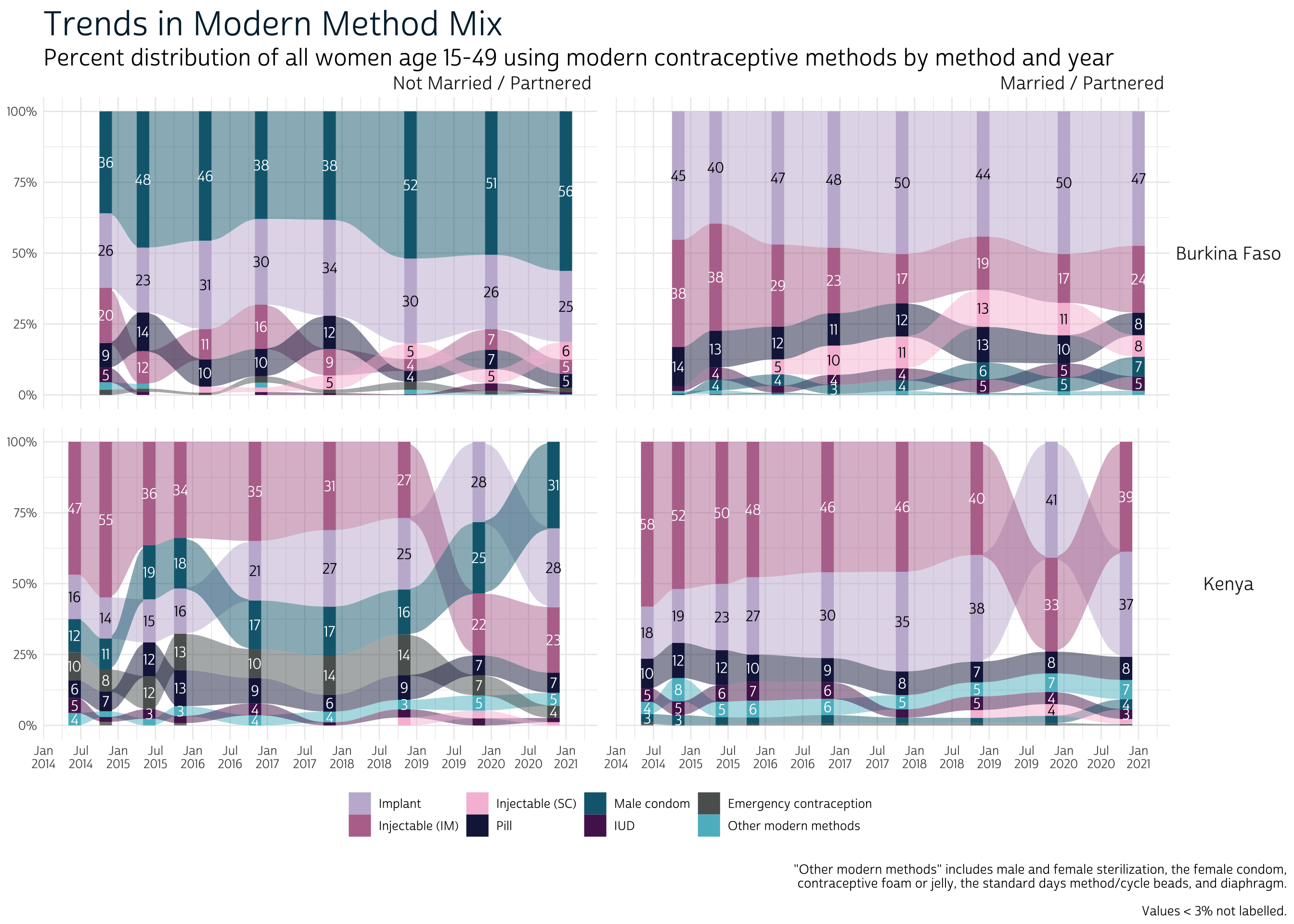
In both countries, there’s quite a big difference in the popularity of modern methods between married / partnered and non-partnered women. Of course, the demand for modern family planning methods is probably very different for women in each of these subgroups. In the next few weeks, we’ll dig deeper into issues surrounding measurement of demand for family planning, and related measures like unmet need.

USAID - Data for Impact ↩︎
IPUMS PMA includes a variable INTFQCMC, but it is not currently available for all samples.↩︎
Not included in the PMA graphic above↩︎

Trends in Modern Contraceptive Method Mix