In our last technical post, we demonstrated how to calculate several different monthly temperature metrics with the ultimate goal of linking these values to individual child records in the 2012 Mali DHS survey.
However, in contrast to the technique we used in our CHIRPS post, we can’t simply join our temperature data onto our DHS sample by enumeration cluster alone because each child in our sample has a different birth date, and therefore different temperature exposure prior to birth.
To account for this, we need to join our temperature data to each child survey record both by enumeration cluster (which contains the spatial information) as well as the child’s birth date (which contains the temporal information).
First, we’ll identify the monthly CHIRTS data corresponding to each of our enumeration cluster areas, producing a time series of temperature values for each cluster. Next, we’ll identify the time series of temperature values for the 9 months prior to each child’s birth and use it to calculate trimester-specific temperature exposure values for each child. Finally, we’ll use the joined data to build a simple model predicting birth weight outcomes from temperature exposure.
This post will build on our previous post where we built several monthly temperature metrics. If you haven’t had the chance to read through that post yet, we encourage you to start there.
Before getting started, we’ll load the necessary packages for this post:
Data
DHS survey data
We will obtain 2012 Mali data from IPUMS DHS. In this extract, we’ve selected the following variables:
-
HEIGHTFEM: Height of woman in centimeters -
KIDSEX: Sex of child -
KIDDOBCMC: Child’s date of birth (CMC) -
BIRTHWT: Birth weight in kilos -
BIRTHWTREF: Source of weight at birth (health card or recall)
Check out our walkthrough for downloading IPUMS DHS data if you need help producing a similar extract.
We’ll load our data using ipumsr:
ml_dhs <- read_ipums_micro("data/idhs_00021.xml")
#> Use of data from IPUMS DHS is subject to conditions including that users should cite the data appropriately. Use command `ipums_conditions()` for more details.

ml_dhs
#> # A tibble: 10,326 × 48
#>    SAMPLE            SAMPLESTR     COUNTRY    YEAR IDHSPID IDHSHID DHSID IDHSPSU
#>    <int+lbl>         <chr+lbl>     <int+lbl> <int> <chr>   <chr>   <chr>   <dbl>
#>  1 46605 [Mali 2012] 46605 [Mali … 466 [Mal…  2012 46605 … 46605 … ML20… 4.66e10
#>  2 46605 [Mali 2012] 46605 [Mali … 466 [Mal…  2012 46605 … 46605 … ML20… 4.66e10
#>  3 46605 [Mali 2012] 46605 [Mali … 466 [Mal…  2012 46605 … 46605 … ML20… 4.66e10
#>  4 46605 [Mali 2012] 46605 [Mali … 466 [Mal…  2012 46605 … 46605 … ML20… 4.66e10
#>  5 46605 [Mali 2012] 46605 [Mali … 466 [Mal…  2012 46605 … 46605 … ML20… 4.66e10
#>  6 46605 [Mali 2012] 46605 [Mali … 466 [Mal…  2012 46605 … 46605 … ML20… 4.66e10
#>  7 46605 [Mali 2012] 46605 [Mali … 466 [Mal…  2012 46605 … 46605 … ML20… 4.66e10
#>  8 46605 [Mali 2012] 46605 [Mali … 466 [Mal…  2012 46605 … 46605 … ML20… 4.66e10
#>  9 46605 [Mali 2012] 46605 [Mali … 466 [Mal…  2012 46605 … 46605 … ML20… 4.66e10
#> 10 46605 [Mali 2012] 46605 [Mali … 466 [Mal…  2012 46605 … 46605 … ML20… 4.66e10
#> # ℹ 10,316 more rows
#> # ℹ 40 more variables: IDHSSTRATA <dbl>, CASEID <chr>, HHID <chr>, PSU <dbl>,
#> #   STRATA <dbl>, DOMAIN <dbl>, HHNUM <dbl>, CLUSTERNO <dbl>, LINENO <int>,
#> #   BIDX <int>, PERWEIGHT <dbl>, KIDWT <dbl>, AWFACTT <dbl>, AWFACTU <dbl>,
#> #   AWFACTR <dbl>, AWFACTE <dbl>, AWFACTW <dbl>, DVWEIGHT <dbl>,
#> #   URBAN <int+lbl>, GEO_ML1987_2018 <int+lbl>, GEO_ML1995_2018 <int+lbl>,
#> #   GEO_ML2012 <int+lbl>, AGE <int>, AGE5YEAR <int+lbl>, RESIDENT <int+lbl>, …
DHS boundaries
We’ll use the Mali borders that we prepared in our previous CHIRTS post. We describe the process there, but we’ve reproduced the code in the following collapsed block if you need to refresh your memory. As a reminder, you can obtain IPUMS integrated geography files from this table.
Border preparation
ml_borders <- read_ipums_sf("data/gps/geo_ml1995_2018.zip")

# Validate internal borders
ml_borders_neat <- st_make_valid(ml_borders)

# Collapse internal borders to get single country border
ml_borders_out <- ml_borders_neat |>
  st_union() |>
  st_simplify(dTolerance = 1000) |>
  st_as_sf()

# Transform to UTM 29N coordinates, buffer, and convert back to WGS84
ml_borders_buffer <- ml_borders_out |>
  st_transform(crs = 32629) |>
  st_buffer(dist = 10000) |>
  st_transform(crs = 4326)
DHS enumeration clusters
We can download the enumeration cluster coordinates from the DHS Program. We first described this process in our CHIRPS post. Simply follow the same instructions, substituting Mali where we previously used Burkina Faso.
You should obtain a file called MLGE6BFL.zip, which can be loaded with read_ipums_sf():
ml_clust <- read_ipums_sf("data/MLGE6BFL.zip")As we’ve done in the past, we’ll buffer our cluster coordinates so we capture the environmental effects of the general region around each survey location
ml_clust_buffer <- ml_clust |>
  st_transform(crs = 32629) |>
  st_buffer(dist = 10000) |>
  st_transform(crs = 4326)
CHIRTS
For this post, we’ll use the monthly heatwave proportions that we calculated at the end of our previous CHIRTS post.
However for the purposes of demonstration, in that post we used a single year of CHIRTS data. Now that we’re planning to attach temperature data to our DHS survey data, we need to consider the full range of birth dates represented in our sample.
Extending CHIRTS time series
The DHS contains records for children born within 5 years of the survey date to women between 15 and 49 years of age. Thus, for the 2012 Mali sample, we will have records for children ranging from 2008-2012. Further, since we want to identify monthly weather records for the time preceding each birth, we will also need to have data for the year prior to the earliest birth in the sample.
That means that for our 2012 Mali sample, we’ll actually need CHIRTS data for 2007-2012.
Fortunately, the pipeline we set up in our previous post can be easily scaled to accommodate additional years of data. Recall that we built a dedicated function to calculate monthly heatwave proportions:
prop_heatwave <- function(temps, thresh, n_seq) {
  # Convert to RLE of days above threshold
  bin_rle <- rle(temps >= thresh)

  # Identify heatwave events based on sequence length
  is_heatwave <- bin_rle$values & (bin_rle$lengths >= n_seq)

  # Count heatwave days and divide by total number of days
  sum(bin_rle$lengths[is_heatwave]) / length(temps)
}
All we need to do, then, is apply this function to input CHIRTS data for 2007 to 2012, rather than just for 2012. To do so, we’ve downloaded all 6 years of data manually as described previously and placed each file in a data/chirts directory.
We can load them by first obtaining the file path to each file with list.files(). Then, we use the familiar rast() to load all 6 files into a single SpatRaster.
chirts_files <- list.files("data/chirts", full.names = TRUE)

ml_chirts <- rast(chirts_files)
As we did last time, we’ll crop the CHIRTS raster to the region directly around Mali:
ml_chirts <- crop(ml_chirts, ml_borders_buffer, snap = "out")Now we can use the tapp() function introduced in our previous post to calculate monthly heatwave proportions for each month/year combination. The only difference here is that we use index = "yearmonths" instead of index = "months" since we have multiple years of data. This ensures that we don’t aggregate months together across years.
# Calculate monthly proportion of heatwave days
ml_chirts_heatwave <- tapp(
  ml_chirts,
  function(x) prop_heatwave(x, thresh = 35, n_seq = 3),
  index = "yearmonths" # New index to account for multiple years
)
As expected, we now have a SpatRaster with 72 layers: one for each month/year combination from 2007-2012. Each layer contains the proportion of days that met our heatwave threshold of 3+ consecutive days exceeding 35°C.
ml_chirts_heatwave
#> class       : SpatRaster
#> size        : 301, 335, 72  (nrow, ncol, nlyr)
#> resolution  : 0.05, 0.05  (x, y)
#> extent      : -12.35, 4.399999, 10.05, 25.1  (xmin, xmax, ymin, ymax)
#> coord. ref. : lon/lat WGS 84
#> source      : ml_chirts_heatwave.nc
#> names       : ml_ch~ave_1, ml_ch~ave_2, ml_ch~ave_3, ml_ch~ave_4, ml_ch~ave_5, ml_ch~ave_6, ...
#> time (ymnts): 2007-Jan to 2012-Dec (72 steps)This post was built using terra 1.7-78. Older versions of terra contain a bug that may produce incorrect time units when index = "yearmonths".
If you’re running an older version of terra, we suggest updating the package with install.packages("terra"). Otherwise, you may be able to temporarily avoid the issue by manually setting the correct time values:
Attach heatwave metrics to DHS survey data
Now that we have our heatwave proportions for the full time range of the children in our DHS sample, we can shift our focus to joining these two data sources.
Reconcile date representations
To deal with the temporal component of the join, we’ll need to identify the relevant months of data for each child in our DHS sample. Each child’s birth date recorded in the KIDDOBCMC variable:
ml_dhs$KIDDOBCMC
#>     [1] 1311 1301 1316 1356 1305 1337 1301 1318 1337 1313 1354 1313 1326 1312
#>    [15] 1330 1316 1354 1311 1335 1338 1305 1321 1305 1347 1315 1354 1309 1323
#>    [29] 1324 1349 1315 1297 1334 1317 1336 1334 1338 1304 1323 1307 1354 1311
....
You might have expected that these would be dates, but we actually have a series of 4-digit numbers. This is because dates are encoded as century month codes in the DHS. A century month code (CMC) encodes time as the number of months that have elapsed since 1900. CMCs are useful for calculating intervals of time, because they can be easily added and subtracted.
However, the time encoded in our CHIRTS heatwave data aren’t encoded in CMC format, so we’ll need to reconcile these two time representations.
Working with CMCs
Since converting between CMCs and traditional dates is a common and well-defined task, we’ll build some helper functions to handle the conversion. That way, we can easily convert back and forth without having to remember the CMC conversion formula each time.
Fortunately, the description of the KIDDOBCMC variable describes the arithmetic required to convert. We’ve translated that text into the following function, which takes an input CMC and converts it to year-month format:
You can view the description for any variable in your extract using the ipums_var_desc() function from ipumsr.
Similarly, we’ll create a function that goes in the reverse direction:
For instance, a CMC of 1307 turns out to be the same as November, 2008:
cmc_to_ym(1307)
#> [1] "2008-11-01"
And vice versa:
ym_to_cmc("2008-11-01")
#> [1] 1307
Now we have an easy way to reconcile the temporal information in our two data sources.
Attaching heatwaves to DHS clusters
To extract the average heatwave proportions for each DHS enumeration cluster, we’ll use terra’s extract(), which we’ve introduced previously.
# Extract mean heatwave proportions for each DHS cluster region
chirts_clust <- extract(
  ml_chirts_heatwave,
  ml_clust_buffer,
  fun = mean,
  weights = TRUE
) |>
  as_tibble()

chirts_clust
#> # A tibble: 413 × 73
#>       ID ml_chirts_heatwave_1 ml_chirts_heatwave_2 ml_chirts_heatwave_3
#>    <int>                <dbl>                <dbl>                <dbl>
#>  1     1                0.210                0.498                0.806
#>  2     2                0.226                0.714                0.903
#>  3     3                0.270                0.910                1
#>  4     4                0.226                0.857                0.968
#>  5     5                0.258                0.898                0.996
#>  6     6                0.226                0.841                0.935
#>  7     7                0.169                0.679                0.903
#>  8     8                0.161                0.5                  0.892
#>  9     9                0.226                0.858                0.973
#> 10    10                0.194                0.627                0.924
#> # ℹ 403 more rows
#> # ℹ 69 more variables: ml_chirts_heatwave_4 <dbl>, ml_chirts_heatwave_5 <dbl>,
#> #   ml_chirts_heatwave_6 <dbl>, ml_chirts_heatwave_7 <dbl>,
#> #   ml_chirts_heatwave_8 <dbl>, ml_chirts_heatwave_9 <dbl>,
#> #   ml_chirts_heatwave_10 <dbl>, ml_chirts_heatwave_11 <dbl>,
#> #   ml_chirts_heatwave_12 <dbl>, ml_chirts_heatwave_13 <dbl>,
#> #   ml_chirts_heatwave_14 <dbl>, ml_chirts_heatwave_15 <dbl>, …
Wide vs. long format
extract() provides data in wide format, where each column represents our temperature values (in this case, mean proportion of heatwave days in a given month) and each row represents a DHS enumeration cluster.
To join on our DHS survey data, we’ll want our data to be in long format, where each row represents a single month of temperature data for a single DHS cluster. We can accomplish this conversion with the pivot_longer() function from the tidyr package.
© RStudio, Inc. (MIT)
First, we’ll rename the columns in our extracted data. Currently, they’re listed in incremental order, which isn’t very intuitive. Instead, we’ll rename them using the CMC code of the month that each column represents. We can use our helper function to convert these dates to CMC format.
We’ll also update the "ID" column to be named "DHSID" for consistency with the name used in the DHS survey to represent the enumeration cluster ID:
Next, we need to convert the incremental ID numbers for each cluster to their corresponding DHSID code. The ID values in chirts_clust represent the clusters extracted from ml_clust in index order. Thus, we simply need to reassign the incremental ID codes in chirts_clust with the IDs in ml_clust.
# Convert index numbers to corresponding DHSID codes
chirts_clust$DHSID <- ml_clust$DHSID

chirts_clust
#> # A tibble: 413 × 73
#>    DHSID  `1285` `1286` `1287` `1288` `1289` `1290`  `1291` `1292` `1293` `1294`
#>    <chr>   <dbl>  <dbl>  <dbl>  <dbl>  <dbl>  <dbl>   <dbl>  <dbl>  <dbl>  <dbl>
#>  1 ML201…  0.210  0.498  0.806  1      1      0.935 0.358        0 0.318   1
#>  2 ML201…  0.226  0.714  0.903  1      0.999  0.825 0.346        0 0.0355  0.857
#>  3 ML201…  0.270  0.910  1      0.999  1      0.604 0            0 0       0.150
#>  4 ML201…  0.226  0.857  0.968  1      1      0.718 0.186        0 0       0.159
#>  5 ML201…  0.258  0.898  0.996  0.988  1      0.599 0            0 0       0.141
#>  6 ML201…  0.226  0.841  0.935  1      1      0.572 0            0 0       0.373
#>  7 ML201…  0.169  0.679  0.903  1      1      0.933 0.305        0 0.427   0.778
#>  8 ML201…  0.161  0.5    0.892  1      1      0.967 0.581        0 0.5     0.901
#>  9 ML201…  0.226  0.858  0.973  0.991  1      0.569 0.00296      0 0       0.144
#> 10 ML201…  0.194  0.627  0.924  1      1      1.000 0.572        0 0.385   0.957
#> # ℹ 403 more rows
#> # ℹ 62 more variables: `1295` <dbl>, `1296` <dbl>, `1297` <dbl>, `1298` <dbl>,
#> #   `1299` <dbl>, `1300` <dbl>, `1301` <dbl>, `1302` <dbl>, `1303` <dbl>,
#> #   `1304` <dbl>, `1305` <dbl>, `1306` <dbl>, `1307` <dbl>, `1308` <dbl>,
#> #   `1309` <dbl>, `1310` <dbl>, `1311` <dbl>, `1312` <dbl>, `1313` <dbl>,
#> #   `1314` <dbl>, `1315` <dbl>, `1316` <dbl>, `1317` <dbl>, `1318` <dbl>,
#> #   `1319` <dbl>, `1320` <dbl>, `1321` <dbl>, `1322` <dbl>, `1323` <dbl>, …
Now we’re ready to convert to long format data. pivot_longer() will convert a set of columns in our wide data to two columns in our long data. The names of these columns will be stored in one of the output columns, and their associated values will be stored in the other.
Below, we indicate that we want to pivot all columns except the DHSID column (the data are already long on DHSID). We also indicate that we want the new column of names to be called "CHIRTSCMC" and the new column of values to be called "PROPHEATWAVE". Finally, we use the names_transform argument to convert all the names to numeric format, so they will be interpretable as CMCs.
# Convert to long format for each cluster/month combination
chirts_clust <- pivot_longer(
  chirts_clust,
  cols = -DHSID,
  names_to = "CHIRTSCMC",
  values_to = "PROPHEATWAVE",
  names_transform = as.numeric
)

chirts_clust
#> # A tibble: 29,736 × 3
#>    DHSID          CHIRTSCMC PROPHEATWAVE
#>    <chr>              <dbl>        <dbl>
#>  1 ML201200000001      1285        0.210
#>  2 ML201200000001      1286        0.498
#>  3 ML201200000001      1287        0.806
#>  4 ML201200000001      1288        1
#>  5 ML201200000001      1289        1
#>  6 ML201200000001      1290        0.935
#>  7 ML201200000001      1291        0.358
#>  8 ML201200000001      1292        0
#>  9 ML201200000001      1293        0.318
#> 10 ML201200000001      1294        1
#> # ℹ 29,726 more rows
As you can see, each row now corresponds to a cluster/month combination, and the corresponding heatwave value is stored in the PROPHEATWAVE column.
Joining on DHS survey data
Before we join our heatwave data on our DHS survey data, we need to do some housekeeping. Some of the variables we want to include in our model include missing values or implied decimals, which we’ll want to clean up before we try to join the DHS survey with our CHIRTS data.
DHS survey data preparation
First, we’ll make a new column that stores a unique ID for each child in the sample by combining the ID for each woman and the index for each of her births. This will make it easier to ensure that we join data independently for each child in the sample:
# str_squish() removes excess whitespace in the ID strings
ml_dhs <- ml_dhs |>
  mutate(KIDID = stringr::str_squish(paste(IDHSPID, BIDX)))
We’ll also want to make sure to recode several of our variables that include missing values. We can check the missing value codes for a variable using ipums_val_labels(). For instance, for our key outcome variable, BIRTHWT, we see that all values over 9996 are missing in some way:
ipums_val_labels(ml_dhs$BIRTHWT)
#> # A tibble: 5 × 2
#>     val lbl
#>   <int> <chr>
#> 1  9995 9995+
#> 2  9996 Not weighed at birth
#> 3  9997 Don't know
#> 4  9998 Missing
#> 5  9999 NIU (not in universe)
Looking at these values, you may be surprised to see 4-digit weights. To investigate further, we can display detailed variable information with ipums_var_desc():
ipums_var_desc(ml_dhs$BIRTHWT)
#> [1] "For children born in the three to five years before the survey, BIRTHWT (M19) reports the child's birthweight in kilos with three implied decimal places (or, alternatively stated, in grams with no decimal places). Children who were not weighed are coded 9996."
Note that the description mentions that there are 3 implied decimal places. So, we’ll recode BIRTHWT to be NA in the cases where the value is more than 9996, and we’ll divide by 1000 otherwise. We’ll do a similar process with a few other variables as well:
In practice, we would likely want to deal with BIRTHWT values of 9995+, which represent all weights above the 9.995 kg threshold. It’s not fully correct to treat these values as equal to 9.995, since their values are actually unknown. This problem is known as censoring, but we won’t address it in this post to keep this demonstration focused on our core goal of integrating environmental data with DHS surveys.
Residency
When working with environmental data, we want to be attentive to the members of the sample who may have recently moved to a location, as recent arrivals likely didn’t experience the previous environmental effects recorded for the area they currently live!
IPUMS DHS includes the RESIDEINTYR variable to indicate how long survey respondents have lived at their current location.
Unfortunately, this variable wasn’t collected for the Mali 2012 sample. However, we do have a record of whether a respondent is a visitor to the location or not. At a minimum, we’ll remove records for those who are listed as visitors, since we can’t be confident that they experienced the environmental data for the cluster their response was recorded in.
ml_dhs <- ml_dhs |>
  filter(RESIDENT == 1)
Data types
Finally, we want to recode our variables to the appropriate data type. In our case, we just need to convert all labeled variables to factors. BIDX is unlabeled, but represents a factor, so we’ll explicitly convert that variable as well:
Attaching data sources
At its simplest, we could join our prepared DHS survey data with our extracted heatwave data by matching records based on their cluster and birth month. We can use left_join() from dplyr to do so. This will retain all records in our DHS survey sample and attach temperature values where the birth date (KIDDOBCMC) is equal to the month of temperature data in chirts_clust:
However, this only attaches a single month of temperature data for each child. What we’d rather have is a time series of values covering the time between conception and birth.
To accomplish this, we can define a new variable, KIDCONCEPTCMC, which contains the CMC of the month 9 months before the birth date.
# Make unique ID for each kid using woman's ID and Birth index
ml_dhs <- ml_dhs |>
  mutate(KIDCONCEPTCMC = KIDDOBCMC - 9)
Now, we want to join all 9 of the relevant monthly temperature records to each child’s DHS survey record. That is, we want to match records that have the same DHSID, a birthdate that is after the CHIRTS data that will be joined, and a conception date that is before the CHIRTS data that will be joined. We can use join_by() from dplyr to specify these more complex criteria:
# Join 9 months of CHIRTS data to each child record
ml_dhs_chirts <- left_join(
  ml_dhs,
  chirts_clust,
  by = join_by(
    DHSID == DHSID, # Cluster ID needs to match
    KIDDOBCMC > CHIRTSCMC, # DOB needs to be after all joined temp. data
    KIDCONCEPTCMC <= CHIRTSCMC # Conception date needs to be before all joined temp. data
  )
)
We should end up with a dataset that contains 9 records for each child: one for each month between their conception and birth. We can confirm by counting the records for each KIDID:
# Each kid should have 9 rows now
ml_dhs_chirts |>
  count(KIDID)
#> # A tibble: 10,300 × 2
#>    KIDID               n
#>    <chr>           <int>
#>  1 46605 1 14 2 1      9
#>  2 46605 1 16 2 1      9
#>  3 46605 1 16 5 1      9
#>  4 46605 1 16 5 2      9
#>  5 46605 1 4 2 1       9
#>  6 46605 1 42 2 1      9
#>  7 46605 1 42 2 2      9
#>  8 46605 1 50 2 1      9
#>  9 46605 1 75 12 1     9
#> 10 46605 1 75 12 2     9
#> # ℹ 10,290 more rows
We can pull out a few columns for an individual child to make it more clear how things are being joined:
# Example of what our data look like for one kid:
ml_dhs_chirts |>
  filter(KIDID == "46605 1 4 2 1") |>
  select(KIDID, DHSID, KIDDOBCMC, CHIRTSCMC, PROPHEATWAVE)
#> # A tibble: 9 × 5
#>   KIDID         DHSID          KIDDOBCMC CHIRTSCMC PROPHEATWAVE
#>   <chr>         <chr>              <dbl>     <dbl>        <dbl>
#> 1 46605 1 4 2 1 ML201200000001      1311      1302       0.822
#> 2 46605 1 4 2 1 ML201200000001      1311      1303       0.103
#> 3 46605 1 4 2 1 ML201200000001      1311      1304       0
#> 4 46605 1 4 2 1 ML201200000001      1311      1305       0.244
#> 5 46605 1 4 2 1 ML201200000001      1311      1306       0.787
#> 6 46605 1 4 2 1 ML201200000001      1311      1307       0.624
#> 7 46605 1 4 2 1 ML201200000001      1311      1308       0
#> 8 46605 1 4 2 1 ML201200000001      1311      1309       0.0968
#> 9 46605 1 4 2 1 ML201200000001      1311      1310       0.741
As we can see, an individual child (KIDID) is associated with heatwave data (PROPHEATWAVE) for each of the 9 CHIRTS months (CHIRTSCMC) prior to their birth date (KIDDOBCMC).
For a different child we’ll get a similar output, but because this child has a different birth date, the specific PROPHEATWAVE values will be different, even if the cluster ID is the same:
ml_dhs_chirts |>
  filter(KIDID == "46605 1255 2 2") |>
  select(KIDID, DHSID, KIDDOBCMC, CHIRTSCMC, PROPHEATWAVE)
#> # A tibble: 9 × 5
#>   KIDID          DHSID          KIDDOBCMC CHIRTSCMC PROPHEATWAVE
#>   <chr>          <chr>              <dbl>     <dbl>        <dbl>
#> 1 46605 1255 2 2 ML201200000001      1305      1296        0
#> 2 46605 1255 2 2 ML201200000001      1305      1297        0
#> 3 46605 1255 2 2 ML201200000001      1305      1298        0.345
#> 4 46605 1255 2 2 ML201200000001      1305      1299        1
#> 5 46605 1255 2 2 ML201200000001      1305      1300        0.999
#> 6 46605 1255 2 2 ML201200000001      1305      1301        1
#> 7 46605 1255 2 2 ML201200000001      1305      1302        0.822
#> 8 46605 1255 2 2 ML201200000001      1305      1303        0.103
#> 9 46605 1255 2 2 ML201200000001      1305      1304        0
Similarly, for a child from a different cluster, we’ll have different PROPHEATWAVE values regardless of which month is under consideration:
ml_dhs_chirts |>
  filter(KIDID == "46605 518171 3 1") |>
  select(KIDID, DHSID, KIDDOBCMC, CHIRTSCMC, PROPHEATWAVE)
#> # A tibble: 9 × 5
#>   KIDID            DHSID          KIDDOBCMC CHIRTSCMC PROPHEATWAVE
#>   <chr>            <chr>              <dbl>     <dbl>        <dbl>
#> 1 46605 518171 3 1 ML201200000518      1314      1305       0.379
#> 2 46605 518171 3 1 ML201200000518      1314      1306       0.877
#> 3 46605 518171 3 1 ML201200000518      1314      1307       0.456
#> 4 46605 518171 3 1 ML201200000518      1314      1308       0
#> 5 46605 518171 3 1 ML201200000518      1314      1309       0.0213
#> 6 46605 518171 3 1 ML201200000518      1314      1310       0.505
#> 7 46605 518171 3 1 ML201200000518      1314      1311       0.923
#> 8 46605 518171 3 1 ML201200000518      1314      1312       1
#> 9 46605 518171 3 1 ML201200000518      1314      1313       1
Now that we have the correct 9-month time series for each child, we can further aggregate to get a trimester-specific exposure metric for each child.
First, we’ll create a TRIMESTER variable, which encodes the trimester that each month belongs to for each child:
Then, we’ll average the heatwave proportions across trimesters for each child:
# Average proportion of heatwave days within each child and trimester
ml_dhs_tri <- ml_dhs_chirts |>
  summarize(
    MEANPROPHEATWAVE = mean(PROPHEATWAVE),
    .by = c(KIDID, TRIMESTER)
  )

ml_dhs_tri
#> # A tibble: 30,900 × 3
#>    KIDID          TRIMESTER MEANPROPHEATWAVE
#>    <chr>          <fct>                <dbl>
#>  1 46605 1 14 2 1 1                    0.439
#>  2 46605 1 14 2 1 2                    0.218
#>  3 46605 1 14 2 1 3                    0.781
#>  4 46605 1 16 2 1 1                    0.240
#>  5 46605 1 16 2 1 2                    0.903
#>  6 46605 1 16 2 1 3                    0.731
#>  7 46605 1 16 5 1 1                    0.944
#>  8 46605 1 16 5 1 2                    0.322
#>  9 46605 1 16 5 1 3                    0.578
#> 10 46605 1 16 5 2 1                    0.115
#> # ℹ 30,890 more rows
We now have 3 records for each child—one for each trimester. Our temperature metric now represents the average monthly proportion of days spent in a heatwave across the three months of each trimester as well as across the spatial region of each buffered cluster region.
Recall that in this case we define a heatwave day as any day belonging to a sequence of at least 3 days over 35°C.
A basic model
To complete this post, we’ll use our prepared data to generate a model predicting birth weight outcomes from heatwave exposure. We’ll interact heatwave exposure with the trimester of exposure to determine whether the effects of heatwave exposure may differ across trimesters.
We’ll also include several covariates and control variables, including child’s sex, mother’s age and height, birth order, education level, and the source of birth weight data.
We’re building this model primarily to demonstrate how you might use aggregated survey and environmental data. It’s not intended to be be a comprehensive modeling approach, and there are likely other variables that should be considered and included.
First, we need to reattach our covariates to our trimester-aggregated data from the previous step. We’ll do so by selecting our variables of interest and joining them back on our heatwave exposure metrics calculated for each trimester and child ID.
# Select covariates of interest. We want a single row of covariates for each
# KIDID
ml_dhs_chirts_sub <- ml_dhs_chirts |>
  select(
    DHSID, IDHSPID, KIDID, KIDSEX, BIDX, EDUCLVL,
    BIRTHWTREF, BIRTHWT, AGE, TRIMESTER, HEIGHTFEM
  ) |>
  distinct() # Remove extra month-level records for each trimester

# Join trimester-aggregated data to covariates
ml_dhs_tri <- full_join(
  ml_dhs_tri,
  ml_dhs_chirts_sub,
  by = c("KIDID", "TRIMESTER")
)
Now, we can build a random effects model using lmer from the lme4 package. We won’t get into all the details of random effects models in this post; for now, it’s enough to know that these models allow you to model a separate intercept for observations that belong to different groups. In this case, we fit separate intercepts for each enumeration area (1 | DHSID). This allows us to account for some of the correlation between child observations from the same spatial area.
heatwave_mod <- lme4::lmer(
  BIRTHWT ~ MEANPROPHEATWAVE * TRIMESTER + KIDSEX + AGE + BIDX +
    EDUCLVL + BIRTHWTREF + HEIGHTFEM + (1 | DHSID),
  data = ml_dhs_tri
)
© Daniel D. Sjoberg et al. (MIT)
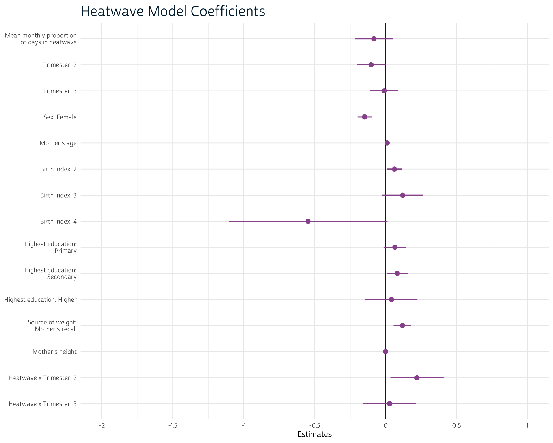
We can summarize our results with the gtsummary package. Based on the confidence intervals reported in this output, it appears that there may be a slight negative relationship between the proportion of heatwave days and birth weight, but the results are not definitive.
The interaction terms suggest that heatwave suggest that the effect of heatwave days on birth weight is slightly more positive in trimester 2 as compared to the effect during trimester 1.
Show table code
library(gtsummary)

tbl_regression(
  heatwave_mod,
  conf.int = TRUE,
  tidy_fun = broom.mixed::tidy,
  label = list(
    MEANPROPHEATWAVE = "Mean proportion of days in heatwave",
    TRIMESTER = "Trimester",
    BIDX = "Birth order",
    EDUCLVL = "Education level",
    BIRTHWTREF = "Birth weight source",
    HEIGHTFEM = "Mother's height (cm)",
    `DHSID.sd__(Intercept)` = "Random effects: Enumeration cluster (SD)",
    `Residual.sd__Observation` = "Random effects: Residual (SD)"
  )
) |>
  italicize_labels() |>
  modify_header(update = list(label = "Covariate")) |>
  as_gt() |>
  gt::tab_header(
    gt::md("# Effects of Heatwave Days on Birthweight")
  )
#> Warning: The `update` argument of `modify_header()` is deprecated as of gtsummary 2.0.0.
#> ℹ Use `modify_header(...)` input instead. Dynamic dots allow for syntax like
#>   `modify_header(!!!list(...))`.
#> ℹ The deprecated feature was likely used in the gtsummary package.
#> Please report the issue at <https://github.com/ddsjoberg/gtsummary/issues>.| Covariate | Beta | 95% CI |
|---|---|---|
| Mean proportion of days in heatwave | -0.08 | -0.22, 0.05 |
| Trimester | ||
| 1 | — | — |
| 2 | -0.10 | -0.20, 0.00 |
| 3 | -0.01 | -0.11, 0.09 |
| Sex of child | ||
| Male | — | — |
| Female | -0.15 | -0.20, -0.10 |
| Age | 0.01 | 0.01, 0.01 |
| Birth order | ||
| 1 | — | — |
| 2 | 0.06 | 0.01, 0.12 |
| 3 | 0.12 | -0.02, 0.26 |
| 4 | -0.55 | -1.1, 0.01 |
| Education level | ||
| No education | — | — |
| Primary | 0.07 | -0.01, 0.14 |
| Secondary | 0.08 | 0.01, 0.16 |
| Higher | 0.04 | -0.14, 0.22 |
| Birth weight source | ||
| From written card | — | — |
| From mother’s recall | 0.12 | 0.06, 0.18 |
| Mother’s height (cm) | 0.00 | 0.00, 0.00 |
| Mean proportion of days in heatwave * Trimester | ||
| Mean proportion of days in heatwave * 2 | 0.22 | 0.03, 0.41 |
| Mean proportion of days in heatwave * 3 | 0.03 | -0.16, 0.21 |
| Random effects: Enumeration cluster (SD) | 0.58 | |
| Random effects: Residual (SD) | 0.82 | |
| Abbreviation: CI = Confidence Interval | ||
We’ve now demonstrated a full workflow to obtain raw CHIRTS raster data, calculate monthly heat exposure metrics, join them on survey records based on the timing of those records, and finally producing a model to understand the impacts of our heatwave definition.
Obviously, for your specific research questions many of these steps will need to change, but we’ve introduced many of the core tools you need when integrating environmental data with DHS surveys. Even if you modify the sources and metrics you use, you should have an understanding of some of the technical considerations that go into this kind of research.
Getting Help
Questions or comments? Check out the IPUMS User Forum or reach out to IPUMS User Support at ipums@umn.edu.