If you’ve visited this blog before, you’ll know that we’re huge fans of the across function form dplyr - that’s because PMA surveys feature a lot of “select all that apply” style questions where each response option gets formatted as a separate binary variable in the IPUMS PMA data extract system. Because we often work with several variables from the same original question, we usually want to apply the same transformations or summary procedures to a group of variables, and across gives us a powerful way to do that.
Sometimes, we might want to use across in the modeling phase of a particular research project. This happens whenever we want to run a batch of similar models with identical controls, but with different dependent variables or key independent variables of interest. Ideally, we’d like to build one generic model formula and use across to substitute key variables in each iteration.
Consider, for example, the kind of research question you might explore with the new PMA Client Exit Interview (CEI) survey from Kenya, where women were asked whether they received counseling on several family planning methods immediately following a visit with their healthcare provider. The IPUMS PMA extract system contains one binary variable for each of these response options:
LCL_201. Which methods were you counselled on during this visit today?
Select all methods mentioned. Be sure to scroll to bottom to see all choices.
You cannot select 'No response' with other options

[] Female sterilization
[] Male sterilization
[] Implant
[] IUD
[] Injectables
[] Pill
[] Emergency contraception
[] Male condom
[] Female condom
[] Diaphragm
[] Foam/Jelly
[] Standard days / cycle beads
[] LAM
[] Rhythm method
[] Withdrawal
[] None of the above
[] No response
You could imagine a situation where a researcher might want to model the odds that a woman received counseling on each one of these methods in turn. You would probably want to control for a number of individual factors like the woman’s age, whether she is married or partnered, and her birth history. These variables would appear in the formula for every model. On the other hand, you might also want to substitute independent variables having to do with the availability, cost, or overall demand for a particular family planning method at the facility she visited. Is there some way we could iterate through all of the family planning methods in this list, substituting both dependent and independent variables relevant to a particular method?
In this post, we’ll showcase an approach to this problem that combines across with pack, a little-known function from the tidyr package that will help us pre-select variables that “go together” in each model. If you visit the documentation page for pack, you’ll see that it’s marked with a blue “maturing” lifecycle tag - this generally means that a particular function is in a stable development stage, but that the package authors are still exploring how it might be used in practice. We think pack offers an excellent way to exploit data masking in certain contexts without need for more advanced tidy-evaluation operators (see rlang). And, because tidyr is part of the “tidyverse”, you’ll be able to load pack and across together in one step:
Setup: join CEI and SDP data
Before we dive in, lets take a look at the complete list variables describing availability, cost, and demand for specific family planning methods at sampled facilities in the most recent round of PMA Service Delivery Point (SDP) surveys. Keep in mind: women were interviewed for CEI surveys at a sampled SDP if that facility had an average daily client volume of at least three family planning clients per day. Any of these SDP variables could be predictors in a model for the likelihood that a client received counseling on a particular method:
There are only 11 base questions associated with the variables in this table, but each question gets repeated once for up to 13 family planning methods included in the SDP survey. You’ll notice that every variable from a particular question shares the same suffix; for example, every variable indicating whether the facility “provides” a method shares the suffix PROV (like CONPROV, CYCBPROV, DIAPROV, etc).
To start, we’ll need to download a data extract containing these variables. In this example, we’ll use an extract that includes only “Facility Respondents” from the Kenya 2019 sample and save it into the “data” folder of our working directory. Load it into R with with ipumsr package like so:
library(ipumsr)

sdp <- read_ipums_micro(
  ddi = "data/pma_00001.xml",
  data = "data/pma_00001.dat.gz"
)
You’ll then need to download a second data extract containing only “Female Respondents” to the 2019 CEI sample from Kenya.
cei <- read_ipums_micro(
  ddi = "data/pma_00002.xml",
  data = "data/pma_00002.dat.gz"
)
In order to link women from the CEI data extract to the correct facility in the SDP data extract, you’ll need to join records by FACILITYID. Here, we will left_join cei with sdp, which means 1) all of the rows in cei will be preserved, and 2) sdp variables for each facility will be copied once for every woman interviewed at that facility. We’ll call the resulting data frame dat.
We mentioned in our CEI Data Discovery post that almost all of the questions on the CEI survey were given only to women who received family planning information or a family planning method during their visit to the facility. You’ll find this information recorded in the variable FPINFOYN, so we’ll drop any case where FPINFOYN == 0, indicating that the woman answered no further questions about family planning services.
A conventional workflow
To keep this example simple, let’s focus our research question on variables related to the availability of a method at the facility where a CEI respondent was interviewed. Specifically, we want to know: are women less likely to receive counseling on a given family planning method if that method is not reliably available from their provider?
Strictly speaking, you don’t need to organize variables into packs to examine this problem. Doing so just makes it easier to manipulate and analyze all of the variables related to a particular family planning method. To see how, let’s lay out a workflow for just one of the family planning methods: we’ll pick IUDs to start.
The CEI variable METHCOUNIUD will be our dependent variable in this example. It indicates whether the woman received any counseling about IUDs during her visit.
# A tibble: 2 × 2
  METHCOUNIUD     n
    <int+lbl> <int>
1     0 [No]   2779
2     1 [Yes]  1122
Our key independent variable should indicate whether the method is “reliably available” at the facility the woman visited. For this example, let’s say that a method is “reliably available” if it was continuously in-stock for three months prior to the SDP interview. You might expect this information to appear in the SDP variable IUDOUT3MO, but look closely at the text from that variable’s universe tab:
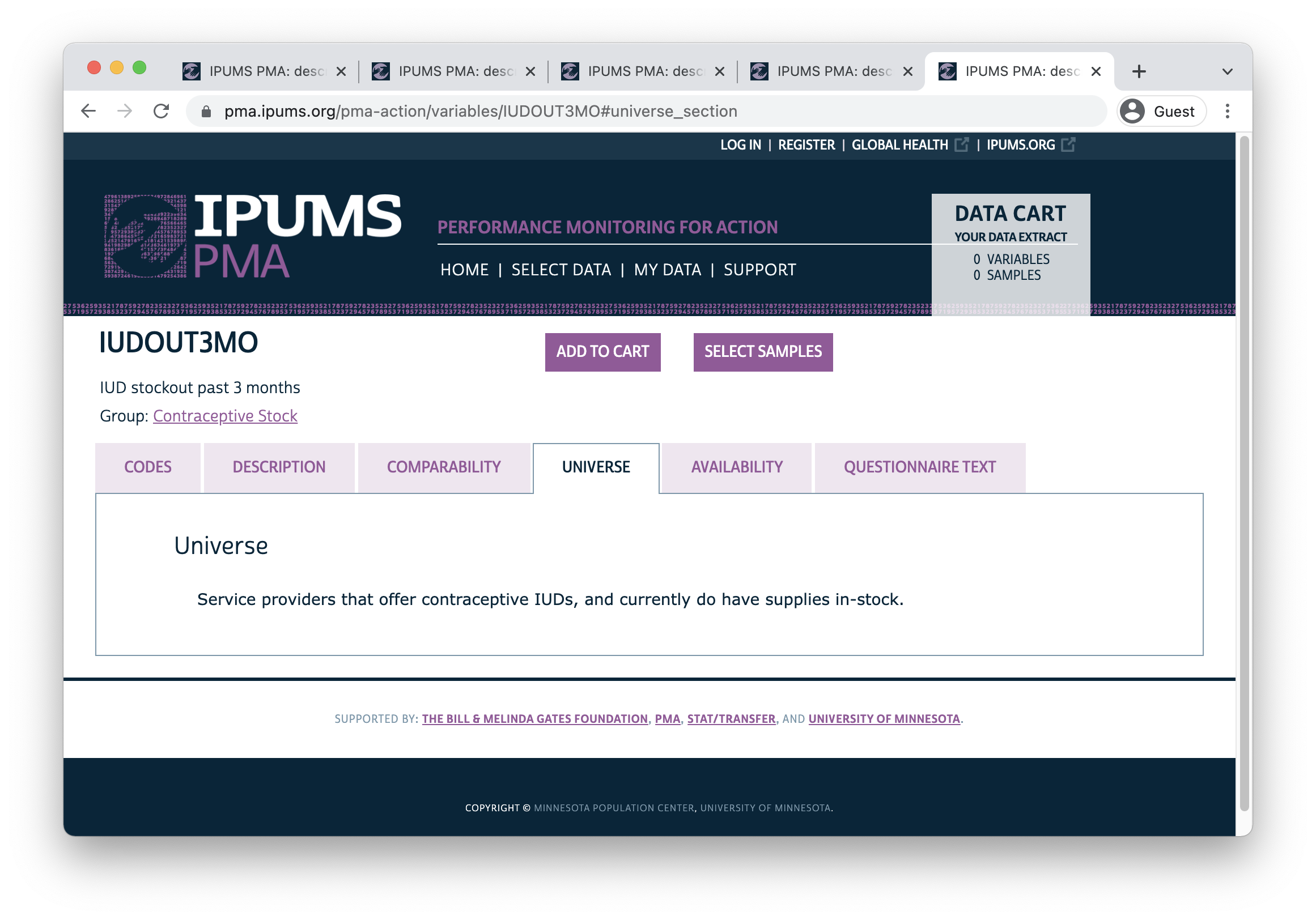
In other words, this question was skipped if 1) a facility that normally provides IUDs was out of stock on the day of the interview, or 2) a facility doesn’t provide the method at all. These cases are marked 99 and labeled NIU (not in universe):
# A tibble: 3 × 2
IUDOUT3MO n
<int+lbl> <int>
1 0 [No] 2980
2 1 [Yes] 204
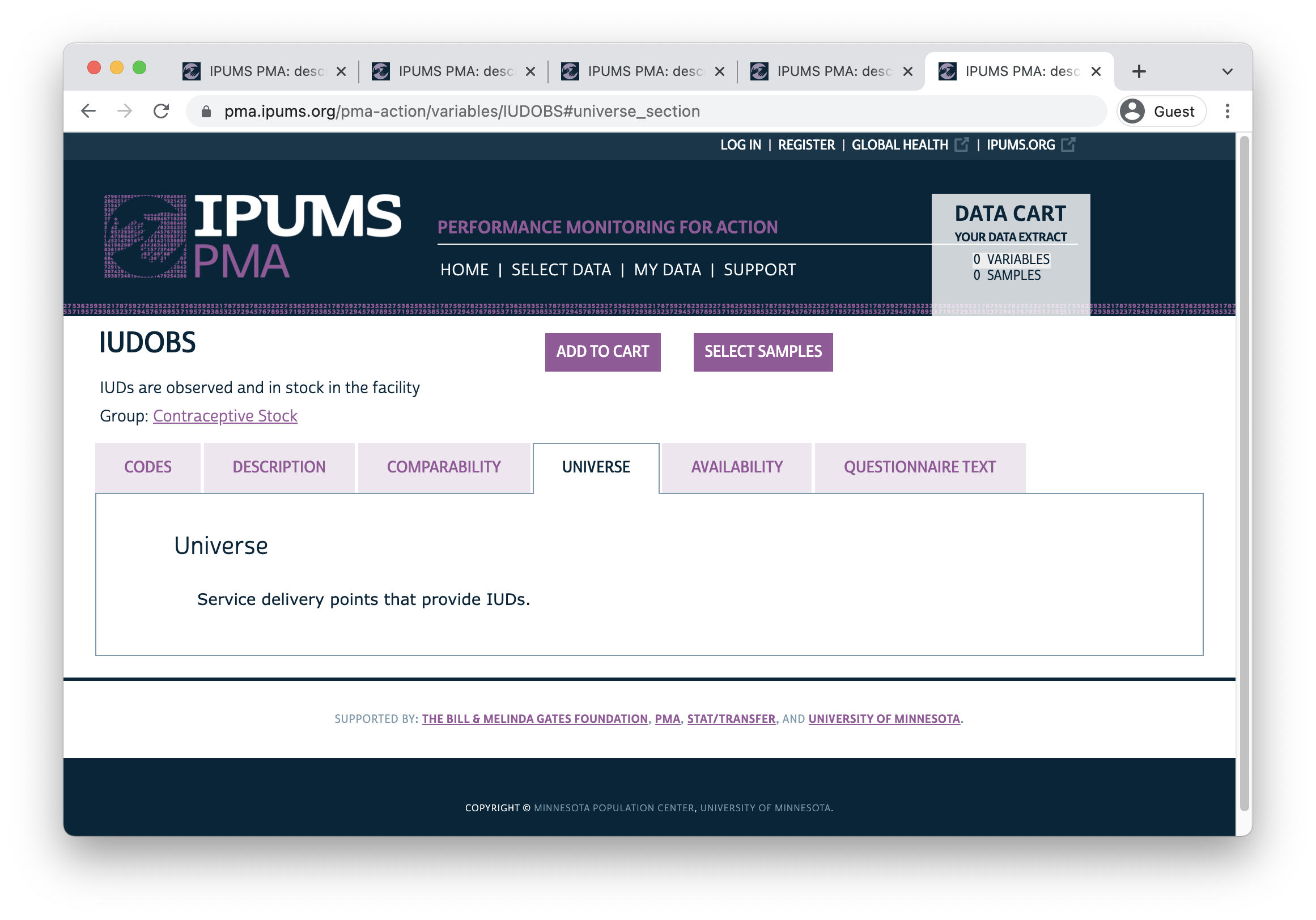
3 99 [NIU (not in universe)] 717We can’t distinguish facilities with temporary stockouts from those that never provide IUDs at all, so we’ll want to combine the information in IUDOUT3MO with another variable. Here, we’ll use IUDOBS, which indicates whether the facility had IUDs in-stock on the day of the SDP interview (and whether that stock was observed directly by the interviewer). In this case, the universe includes all facilities that normally provide IUDs.
# A tibble: 6 × 3
                   IUDOUT3MO                         IUDOBS     n
                   <int+lbl>                      <int+lbl> <int>
1  0 [No]                     1 [In-stock and observed]      2725
2  0 [No]                     2 [In-stock but not observed]   255
3  1 [Yes]                    1 [In-stock and observed]       159
4  1 [Yes]                    2 [In-stock but not observed]    45
5 99 [NIU (not in universe)]  3 [Out of stock]                190
6 99 [NIU (not in universe)] 99 [NIU (not in universe)]       527
Only 190 of the 717 facilities that were NIU (not in universe) for IUDOUT3MO were excluded because of a current stockout. The remaining 527 facilities don’t provide IUDs at all.
Suppose that you were going to combine these variables to build a factor we’ll call IUDAVAIL with 3 levels: facilities where IUDs are “reliably available”, those with a “current or recent stockout”, and those where IUDs are “not provided”. Alone, this task is not too difficult with help from case_when:
dat %>%
  mutate(IUDAVAIL = case_when(
   IUDOBS == 99 ~ "not provided",
   IUDOBS == 3 | IUDOUT3MO == 1 ~ "cur/rec stockout",
   IUDOUT3MO == 0 ~ "reliably avail"
  )) %>%
  count(IUDOBS, IUDOUT3MO, IUDAVAIL)
# A tibble: 6 × 4
                          IUDOBS          IUDOUT3MO IUDAVAIL         n
                       <int+lbl>          <int+lbl> <chr>        <int>
1  1 [In-stock and observed]      0 [No]            reliably av…  2725
2  1 [In-stock and observed]      1 [Yes]           cur/rec sto…   159
3  2 [In-stock but not observed]  0 [No]            reliably av…   255
4  2 [In-stock but not observed]  1 [Yes]           cur/rec sto…    45
5  3 [Out of stock]              99 [NIU (not in u… cur/rec sto…   190
6 99 [NIU (not in universe)]     99 [NIU (not in u… not provided   527
But what should you do if you want to build a similar variable for each of the nine relevant family planning methods? With the approach we’ve used so far, you’d need to write a separate case_when function for every family planning method. Each would look nearly identical to the last, except that you’d use the relevant OBS and OUT3MO variable for each method. Before we explore an approach with pack, take a look at the code we’re hoping to avoid:
dat <- dat %>%
  mutate(
    IUDAVAIL = case_when(
      IUDOBS == 99 ~ "not provided",
      IUDOBS == 3 | IUDOUT3MO == 1 ~ "cur/rec stockout",
      IUDOUT3MO == 0 ~ "reliably avail"
    ),
    CONAVAIL = case_when(
      CONOBS == 99 ~ "not provided",
      CONOBS == 3 | CONOUT3MO == 1 ~ "cur/rec stockout",
      CONOUT3MO == 0 ~ "reliably avail"
    ),
    BEADSAVAIL = case_when(
      CYCBOBS == 99 ~ "not provided",
      CYCBOBS == 3 | CYCBOUT3MO == 1 ~ "cur/rec stockout",
      CYCBOUT3MO == 0 ~ "reliably avail"
    ),
    DIAAVAIL = case_when(
      DIAOBS == 99 ~ "not provided",
      DIAOBS == 3 | DIAOUT3MO == 1 ~ "cur/rec stockout",
      DIAOUT3MO == 0 ~ "reliably avail"
    ),
    EMRGAVAIL = case_when(
      EMRGOBS == 99 ~ "not provided",
      EMRGOBS == 3 | EMRGOUT3MO == 1 ~ "cur/rec stockout",
      EMRGOUT3MO == 0 ~ "reliably avail"
    ),
    FCAVAIL = case_when(
      FCOBS == 99 ~ "not provided",
      FCOBS == 3 | FCOUT3MO == 1 ~ "cur/rec stockout",
      FCOUT3MO == 0 ~ "reliably avail"
    ),
    FJAVAIL = case_when(
      FJOBS == 99 ~ "not provided",
      FJOBS == 3 | FJOUT3MO == 1 ~ "cur/rec stockout",
      FJOUT3MO == 0 ~ "reliably avail"
    ),
    IMPAVAIL = case_when(
      IMPOBS == 99 ~ "not provided",
      IMPOBS == 3 | IMPOUT3MO == 1 ~ "cur/rec stockout",
      IMPOUT3MO == 0 ~ "reliably avail"
    ),
    PILLAVAIL = case_when(
      PILLOBS == 99 ~ "not provided",
      PILLOBS == 3 | PILLOUT3MO == 1 ~ "cur/rec stockout",
      PILLOUT3MO == 0 ~ "reliably avail"
    )
  )
That’s a lot of repeated effort, and a lot places where you might make a simple copy / paste error. And then, imagine repeating this entire process to include the SDP variables related to cost and demand for different methods - you’d have to do another set of nine case_when functions for every variable you wanted to create!
Introducing pack
The difference with pack is that we’ll pre-select all of the variables that we ultimately want to substitute into a method-specific model. In other words, we’ll be manually identifying all of the dependent and key independent variables that “go together” in one step at the beginning of our workflow.
dat_packed <- dat %>%
  pack(
    BEADS = c(METHCOUNBEADS, CYCBOBS, CYCBOUT3MO),
    CON = c(METHCOUNMC, CONOBS, CONOUT3MO),
    DIA = c(METHCOUNDIA, DIAOBS, DIAOUT3MO),
    EMRG = c(METHCOUNEC, EMRGOBS, DIAOUT3MO),
    FC = c(METHCOUNFC, FCOBS, FCOUT3MO),
    FOAM = c(METHCOUNFOAM, FJOBS, FJOUT3MO),
    IMP = c(METHCOUNIMP, IMPOBS, IMPOUT3MO),
    IUD = c(METHCOUNIUD, IUDOBS, IUDOUT3MO),
    PILL = c(METHCOUNPILL, PILLOBS, PILLOUT3MO)
  )
When we do this, we create one tidy data frame - a tibble - for all of the variables dealing with a particular family planning method. Each one of these smaller data frames is “packed” into a single column in the larger parent data frame we’ve called dat_packed. This parent also contains all of the original dat variables that we didn’t happen to include in a pack.
You can call any one of these smaller packs using the same $ operator you’d use to call any other variable.
dat_packed$IUD
# A tibble: 3,901 × 3
   METHCOUNIUD                    IUDOBS IUDOUT3MO
     <int+lbl>                 <int+lbl> <int+lbl>
 1      0 [No] 1 [In-stock and observed]   0 [No]
 2      0 [No] 1 [In-stock and observed]   0 [No]
 3      0 [No] 1 [In-stock and observed]   1 [Yes]
 4      0 [No] 1 [In-stock and observed]   0 [No]
 5      0 [No] 1 [In-stock and observed]   0 [No]
 6      0 [No] 1 [In-stock and observed]   0 [No]
 7      0 [No] 1 [In-stock and observed]   0 [No]
 8      0 [No] 1 [In-stock and observed]   0 [No]
 9      0 [No] 1 [In-stock and observed]   1 [Yes]
10      0 [No] 1 [In-stock and observed]   1 [Yes]
# … with 3,891 more rows
If you call one of these packs in the larger context of its parent data frame, you’ll notice something strange about the output. Let’s call the IUD pack together with FACILITYID:
# A tibble: 3,901 × 2
   FACILITYID IUD$METHCOUNIUD                   $IUDOBS $IUDOUT3MO
    <dbl+lbl>       <int+lbl>                 <int+lbl>  <int+lbl>
 1  404111003          0 [No] 1 [In-stock and observed]    0 [No]
 2  404111003          0 [No] 1 [In-stock and observed]    0 [No]
 3  404111001          0 [No] 1 [In-stock and observed]    1 [Yes]
 4  404111003          0 [No] 1 [In-stock and observed]    0 [No]
 5  404111003          0 [No] 1 [In-stock and observed]    0 [No]
 6  404111003          0 [No] 1 [In-stock and observed]    0 [No]
 7  404111003          0 [No] 1 [In-stock and observed]    0 [No]
 8  404111003          0 [No] 1 [In-stock and observed]    0 [No]
 9  404111001          0 [No] 1 [In-stock and observed]    1 [Yes]
10  404111001          0 [No] 1 [In-stock and observed]    1 [Yes]
# … with 3,891 more rows
The tibble header tells us we’ve printed a tibble with 3,901 rows and 2 columns, but we actually see 4 columns - FACILITYID and each of the 3 variables in our IUD pack. Moreover, the pack name IUD appears as a prefix only on the first column IUD$METHCOUNIUD; the others use $ as shorthand to show that they’re members of the same pack.
In practice, you’ll rarely want to select individual packs by name - it’s much more useful to select and then mutate or summarize all packs at once. You can do this by selecting all variables that are members of the tibble class with where(is_tibble):
# A tibble: 3,901 × 9
   BEADS$METHCOUNBEADS   $CYCBOBS  $CYCBOUT3MO CON$METHCOUNMC  $CONOBS
             <int+lbl>  <int+lbl>    <int+lbl>      <int+lbl> <int+lb>
 1              0 [No] 99 [NIU (… 99 [NIU (no…         0 [No] 1 [In-s…
 2              0 [No] 99 [NIU (… 99 [NIU (no…         0 [No] 1 [In-s…
 3              0 [No] 99 [NIU (… 99 [NIU (no…         0 [No] 1 [In-s…
 4              0 [No] 99 [NIU (… 99 [NIU (no…         0 [No] 1 [In-s…
 5              0 [No] 99 [NIU (… 99 [NIU (no…         0 [No] 1 [In-s…
 6              0 [No] 99 [NIU (… 99 [NIU (no…         0 [No] 1 [In-s…
 7              0 [No] 99 [NIU (… 99 [NIU (no…         0 [No] 1 [In-s…
 8              0 [No] 99 [NIU (… 99 [NIU (no…         0 [No] 1 [In-s…
 9              0 [No] 99 [NIU (… 99 [NIU (no…         0 [No] 1 [In-s…
10              0 [No] 99 [NIU (… 99 [NIU (no…         0 [No] 1 [In-s…
# … with 3,891 more rows, and 7 more variables: DIA <tibble[,3]>,
#   EMRG <tibble[,3]>, FC <tibble[,3]>, FOAM <tibble[,3]>,
#   IMP <tibble[,3]>, IUD <tibble[,3]>, PILL <tibble[,3]>
Using across with packs
Once you’re able to create and select packs, the next step is to repeat the same changes or analytic functions within each pack using across. First, we’ll strip all references to each family planning method from the variable names in each pack with rename. You don’t have to worry about creating duplicate names (e.g. nine variables named OBS) as long as they’re organized in packs (BEADS$OBS, DIA$OBS, EMRG$OBS, etc). In fact, this is exactly what we want!
dat_packed <- dat_packed %>%
  mutate(across(
    where(is_tibble),
    ~.x %>%
      rename(
        COUNSEL = contains("METHCOUN"),
        OBS = contains("OBS"),
        OUT3MO = contains("OUT3MO")
      )
  ))

# Within each pack, you'll now find 3 variables of the same name
dat_packed %>% select(where(is_tibble))
# A tibble: 3,901 × 9
   BEADS$COUNSEL        $OBS     $OUT3MO CON$COUNSEL      $OBS $OUT3MO
       <int+lbl>   <int+lbl>   <int+lbl>   <int+lbl> <int+lbl> <int+l>
 1        0 [No] 99 [NIU (n… 99 [NIU (n…      0 [No] 1 [In-st…  0 [No]
 2        0 [No] 99 [NIU (n… 99 [NIU (n…      0 [No] 1 [In-st…  0 [No]
 3        0 [No] 99 [NIU (n… 99 [NIU (n…      0 [No] 1 [In-st…  0 [No]
 4        0 [No] 99 [NIU (n… 99 [NIU (n…      0 [No] 1 [In-st…  0 [No]
 5        0 [No] 99 [NIU (n… 99 [NIU (n…      0 [No] 1 [In-st…  0 [No]
 6        0 [No] 99 [NIU (n… 99 [NIU (n…      0 [No] 1 [In-st…  0 [No]
 7        0 [No] 99 [NIU (n… 99 [NIU (n…      0 [No] 1 [In-st…  0 [No]
 8        0 [No] 99 [NIU (n… 99 [NIU (n…      0 [No] 1 [In-st…  0 [No]
 9        0 [No] 99 [NIU (n… 99 [NIU (n…      0 [No] 1 [In-st…  0 [No]
10        0 [No] 99 [NIU (n… 99 [NIU (n…      0 [No] 1 [In-st…  0 [No]
# … with 3,891 more rows, and 7 more variables: DIA <tibble[,3]>,
#   EMRG <tibble[,3]>, FC <tibble[,3]>, FOAM <tibble[,3]>,
# IMP <tibble[,3]>, IUD <tibble[,3]>, PILL <tibble[,3]>This makes it easy to apply the same case_when function to each pack.
dat_packed <- dat_packed %>%
  mutate(across(
    where(is_tibble),
    ~.x %>%
      mutate(
        AVAIL = fct_relevel(
          case_when(
            OBS == 99 ~ "not provided",
            OBS == 3 | OUT3MO == 1 ~ "cur/rec stockout",
            OUT3MO == 0 ~ "reliably avail"
          ),
          "reliably avail" # set reference group
        )
      )
  ))

# One `AVAIL` variable was added to each pack
dat_packed %>% select(where(is_tibble))
# A tibble: 3,901 × 9
   BEADS$COUNSEL      $OBS  $OUT3MO $AVAIL CON$COUNSEL    $OBS $OUT3MO
       <int+lbl> <int+lbl> <int+lb> <fct>    <int+lbl> <int+l> <int+l>
 1        0 [No] 99 [NIU … 99 [NIU… not p…      0 [No] 1 [In-…  0 [No]
 2        0 [No] 99 [NIU … 99 [NIU… not p…      0 [No] 1 [In-…  0 [No]
 3        0 [No] 99 [NIU … 99 [NIU… not p…      0 [No] 1 [In-…  0 [No]
 4        0 [No] 99 [NIU … 99 [NIU… not p…      0 [No] 1 [In-…  0 [No]
 5        0 [No] 99 [NIU … 99 [NIU… not p…      0 [No] 1 [In-…  0 [No]
 6        0 [No] 99 [NIU … 99 [NIU… not p…      0 [No] 1 [In-…  0 [No]
 7        0 [No] 99 [NIU … 99 [NIU… not p…      0 [No] 1 [In-…  0 [No]
 8        0 [No] 99 [NIU … 99 [NIU… not p…      0 [No] 1 [In-…  0 [No]
 9        0 [No] 99 [NIU … 99 [NIU… not p…      0 [No] 1 [In-…  0 [No]
10        0 [No] 99 [NIU … 99 [NIU… not p…      0 [No] 1 [In-…  0 [No]
# … with 3,891 more rows, and 7 more variables: DIA <tibble[,4]>,
#   EMRG <tibble[,4]>, FC <tibble[,4]>, FOAM <tibble[,4]>,
#   IMP <tibble[,4]>, IUD <tibble[,4]>, PILL <tibble[,4]>
Modeling with packs
Here’s the real payoff: once you’ve assigned the same name to all of the variables repeated across packs, it’s particularly easy to build parallel model formulas without needing to reference each family planning method by name.
Let’s now use the AVAIL variable for each method to predict the likelihood that a woman would have received counseling on that method in COUNSEL. In other words, we want to build nine logistic regression models using the appropriate pair of method-specific variables.
Before we get to the “packed” approach, again consider a conventional approach where you’d substitute the relevant variables for each family planning method by hand. Have you ever written something that looks like this?
dat %>%
  mutate(across(
    ends_with("AVAIL") & where(is.character),
    ~.x %>% fct_relevel("reliably avail") # set reference group
  )) %>%
  summarise(
    # We want to avoid writing a unique formula for each model if possible:
    BEADS = glm(METHCOUNBEADS ~ BEADSAVAIL, "binomial", cur_data()) %>%
      broom::tidy(exp = TRUE) %>%
      list(),
    CON = glm(METHCOUNMC ~ CONAVAIL, "binomial", cur_data()) %>%
      broom::tidy(exp = TRUE) %>%
      list(),
    DIA = glm(METHCOUNDIA ~ DIAAVAIL, "binomial", cur_data()) %>%
      broom::tidy(exp = TRUE) %>%
      list(),
    EMRG = glm(METHCOUNEC ~ EMRGAVAIL, "binomial", cur_data()) %>%
      broom::tidy(exp = TRUE) %>%
      list(),
    FC = glm(METHCOUNFC ~ FCAVAIL, "binomial", cur_data()) %>%
      broom::tidy(exp = TRUE) %>%
      list(),
    FOAM = glm(METHCOUNFOAM ~ FJAVAIL, "binomial", cur_data()) %>%
      broom::tidy(exp = TRUE) %>%
      list(),
    IMP = glm(METHCOUNIMP ~ IMPAVAIL, "binomial", cur_data()) %>%
      broom::tidy(exp = TRUE) %>%
      list(),
    IUD = glm(METHCOUNIUD ~ IUDAVAIL, "binomial", cur_data()) %>%
      broom::tidy(exp = TRUE) %>%
      list(),
    PILL = glm(METHCOUNPILL ~ PILLAVAIL, "binomial", cur_data()) %>%
      broom::tidy(exp = TRUE) %>%
      list()
  ) %>%
  pivot_longer(everything(), names_to = "COUNSELED") %>%
  unnest(value) %>%
  mutate(across(where(is.double), ~round(.x, 2)))
# A tibble: 26 × 6
   COUNSELED term                 estimate std.error statistic p.value
   <chr>     <chr>                   <dbl>     <dbl>     <dbl>   <dbl>
 1 BEADS     (Intercept)           1   e-2      0.23    -19.0     0
 2 BEADS     BEADSAVAILcur/rec …   2.14e+0      0.42      1.8     0.07
 3 BEADS     BEADSAVAILnot prov…   2.16e+0      0.26      2.97    0
 4 CON       (Intercept)           2.1 e-1      0.05    -34.3     0
 5 CON       CONAVAILcur/rec st…   1.25e+0      0.12      1.85    0.06
 6 CON       CONAVAILnot provid…   0          280.       -0.05    0.96
 7 DIA       (Intercept)           0          822.       -0.02    0.98
 8 DIA       DIAAVAILcur/rec st…   1   e+0   1615.        0       1
 9 DIA       DIAAVAILnot provid…   1.72e+6    822.        0.02    0.99
10 EMRG      (Intercept)           6   e-2      0.09    -29.3     0
# … with 16 more rows
Again - there’s nothing wrong this output. But, with the packed approach we’ll be able to 1) easily substitute method-specific variables in each model without repeating ourselves, and 2) we can use pack names for each model in the COUNSELED column while removing extra text from the term column.
dat_packed %>%
  summarise(across(
    where(is_tibble),
    ~glm(COUNSEL ~ AVAIL, "binomial", .x) %>%
      broom::tidy(exp = TRUE) %>%
      list()
  )) %>%
  pivot_longer(everything(), names_to = "COUNSELED") %>%
  unnest(value) %>%
  mutate(across(where(is.double), ~round(.x, 2))) %>%
  mutate(term = term %>% str_remove("AVAIL"))
# A tibble: 26 × 6
   COUNSELED term               estimate std.error statistic p.value
   <chr>     <chr>                 <dbl>     <dbl>     <dbl>   <dbl>
 1 BEADS     (Intercept)            0.01      0.23    -19.0     0
 2 BEADS     cur/rec stockout       2.14      0.42      1.8     0.07
 3 BEADS     not provided           2.16      0.26      2.97    0
 4 CON       (Intercept)            0.21      0.05    -34.3     0
 5 CON       cur/rec stockout       1.25      0.12      1.85    0.06
 6 CON       not provided           0       280.       -0.05    0.96
 7 DIA       (Intercept)            0       822.       -0.02    0.98
 8 DIA       cur/rec stockout       1      1615.        0       1
 9 DIA       not provided     1722429.      822.        0.02    0.99
10 EMRG      (Intercept)            0.13      0.48     -4.26    0
# … with 16 more rows
What happened here? In summary, we created one pack of variables for each family planning method. We then made all variable names identical across packs so that every pack contains a pair of variables called COUNSEL and AVAIL. Finally, we used across to iterate over every pack via where(is_tibble): we applied the same general glm call to every pack, referenced in the context of a particular iteration with the pronoun .x.
The parent data frame
Now suppose we wanted to introduce a common set of controls with each model. We mentioned at the beginning of this post that we might want to control for certain individual factors like like the woman’s age (AGE), whether she is married or partnered (MARSTAT, recoded here as PARTNERED), and her birth history (BIRTHEVENT).
Remember that these variables were not included in the packed data frames we created above. Instead, they’re located in a parent data frame together with all of our packs. When we iterate through each pack with across, R searches for variables called COUNSEL and AVAIL in one particular pack, masking those in the other packs - this is what allows us to reuse the same variable names for each family planning method. Because each iteration focuses on the contents of one pack, you might expect to get an error if you reference variables outside of that pack.
Fortunately, this is not the case! You can simply add the variables AGE, PARTNERED, and BIRTHEVENT to the formula applied to each pack. R won’t find those variables within the current pack, but it will find them in the parent data frame in which the pack is a member:
dat_packed %>%
  mutate(PARTNERED = MARSTAT %in% 21:22) %>%
  summarise(across(
    where(is_tibble),
    # You can select variables both within and outside of each pack
    ~glm(COUNSEL ~ AVAIL + AGE + PARTNERED + BIRTHEVENT, "binomial", .x) %>%
      broom::tidy(exp = TRUE) %>%
      list()
  )) %>%
  pivot_longer(everything(), names_to = "COUNSELED") %>%
  unnest(value) %>%
  mutate(across(where(is.double), ~round(.x, 2))) %>%
  mutate(term = term %>% str_remove("AVAIL") %>% str_remove("TRUE"))
# A tibble: 53 × 6
   COUNSELED term             estimate std.error statistic p.value
   <chr>     <chr>               <dbl>     <dbl>     <dbl>   <dbl>
 1 BEADS     (Intercept)          0.02      0.56     -7.5     0
 2 BEADS     cur/rec stockout     2.17      0.42      1.82    0.07
 3 BEADS     not provided         2.22      0.26      3.07    0
 4 BEADS     AGE                  1.01      0.02      0.32    0.75
 5 BEADS     PARTNERED            1.34      0.31      0.93    0.35
 6 BEADS     BIRTHEVENT           0.8       0.09     -2.51    0.01
 7 CON       (Intercept)          0.4       0.2      -4.7     0
 8 CON       cur/rec stockout     1.25      0.12      1.85    0.06
 9 CON       not provided         0       279.       -0.05    0.96
10 CON       AGE                  0.99      0.01     -1.48    0.14
# … with 43 more rows
Unpacking
Occasionally, you may want to unpack variables and return your data frame to its original shape. If you’ve duplicated variable names across packs as we’ve done above, you’ll get an error if you unpack without specifying some way to maintain unique names in the reshaped data frame:
Error: Names must be unique.
x These names are duplicated:
  * "COUNSEL" at locations 411, 415, 419, 423, 427, etc.
  * "OBS" at locations 412, 416, 420, 424, 428, etc.
  * "OUT3MO" at locations 413, 417, 421, 425, 429, etc.
  * "AVAIL" at locations 414, 418, 422, 426, 430, etc.
ℹ Use argument `names_repair` to specify repair strategy.
In our case, we’ll use the pack name as a prefix for each new variable name. We’ll use names_sep = "_" to separate each prefix with an underscore:
# A tibble: 3,901 × 36
   BEADS_COUNSEL     BEADS_OBS    BEADS_OUT3MO BEADS_AVAIL CON_COUNSEL
       <int+lbl>     <int+lbl>       <int+lbl> <fct>         <int+lbl>
 1        0 [No] 99 [NIU (not… 99 [NIU (not i… not provid…      0 [No]
 2        0 [No] 99 [NIU (not… 99 [NIU (not i… not provid…      0 [No]
 3        0 [No] 99 [NIU (not… 99 [NIU (not i… not provid…      0 [No]
 4        0 [No] 99 [NIU (not… 99 [NIU (not i… not provid…      0 [No]
 5        0 [No] 99 [NIU (not… 99 [NIU (not i… not provid…      0 [No]
 6        0 [No] 99 [NIU (not… 99 [NIU (not i… not provid…      0 [No]
 7        0 [No] 99 [NIU (not… 99 [NIU (not i… not provid…      0 [No]
 8        0 [No] 99 [NIU (not… 99 [NIU (not i… not provid…      0 [No]
 9        0 [No] 99 [NIU (not… 99 [NIU (not i… not provid…      0 [No]
10        0 [No] 99 [NIU (not… 99 [NIU (not i… not provid…      0 [No]
# … with 3,891 more rows, and 31 more variables: CON_OBS <int+lbl>,
#   CON_OUT3MO <int+lbl>, CON_AVAIL <fct>, DIA_COUNSEL <int+lbl>,
#   DIA_OBS <int+lbl>, DIA_OUT3MO <int+lbl>, DIA_AVAIL <fct>,
#   EMRG_COUNSEL <int+lbl>, EMRG_OBS <int+lbl>,
#   EMRG_OUT3MO <int+lbl>, EMRG_AVAIL <fct>, FC_COUNSEL <int+lbl>,
#   FC_OBS <int+lbl>, FC_OUT3MO <int+lbl>, FC_AVAIL <fct>,
#   FOAM_COUNSEL <int+lbl>, FOAM_OBS <int+lbl>, …
Just the code, please
In case the benefits we gained with pack aren’t quite clear, let’s take a look at the complete workflow in one big code chunk. For comparison’s sake, this is life without pack:
Conventional workflow
dat %>%
  mutate(
    # The "availability" of every family planning method is coded separately
    IUDAVAIL = case_when(
      IUDOBS == 99 ~ "not provided",
      IUDOBS == 3 | IUDOUT3MO == 1 ~ "cur/rec stockout",
      IUDOUT3MO == 0 ~ "reliably avail"
    ),
    CONAVAIL = case_when(
      CONOBS == 99 ~ "not provided",
      CONOBS == 3 | CONOUT3MO == 1 ~ "cur/rec stockout",
      CONOUT3MO == 0 ~ "reliably avail"
    ),
    BEADSAVAIL = case_when(
      CYCBOBS == 99 ~ "not provided",
      CYCBOBS == 3 | CYCBOUT3MO == 1 ~ "cur/rec stockout",
      CYCBOUT3MO == 0 ~ "reliably avail"
    ),
    DIAAVAIL = case_when(
      DIAOBS == 99 ~ "not provided",
      DIAOBS == 3 | DIAOUT3MO == 1 ~ "cur/rec stockout",
      DIAOUT3MO == 0 ~ "reliably avail"
    ),
    EMRGAVAIL = case_when(
      EMRGOBS == 99 ~ "not provided",
      EMRGOBS == 3 | EMRGOUT3MO == 1 ~ "cur/rec stockout",
      EMRGOUT3MO == 0 ~ "reliably avail"
    ),
    FCAVAIL = case_when(
      FCOBS == 99 ~ "not provided",
      FCOBS == 3 | FCOUT3MO == 1 ~ "cur/rec stockout",
      FCOUT3MO == 0 ~ "reliably avail"
    ),
    FJAVAIL = case_when(
      FJOBS == 99 ~ "not provided",
      FJOBS == 3 | FJOUT3MO == 1 ~ "cur/rec stockout",
      FJOUT3MO == 0 ~ "reliably avail"
    ),
    IMPAVAIL = case_when(
      IMPOBS == 99 ~ "not provided",
      IMPOBS == 3 | IMPOUT3MO == 1 ~ "cur/rec stockout",
      IMPOUT3MO == 0 ~ "reliably avail"
    ),
    PILLAVAIL = case_when(
      PILLOBS == 99 ~ "not provided",
      PILLOBS == 3 | PILLOUT3MO == 1 ~ "cur/rec stockout",
      PILLOUT3MO == 0 ~ "reliably avail"
    ),
    across(
      ends_with("AVAIL") & where(is.character),
      ~.x %>% fct_relevel("reliably avail") # set reference group
    ),
    PARTNERED = MARSTAT %in% 21:22
  ) %>%
  # Variables for every family planning method are substituted manually
  summarise(
    BEADS = glm(
      METHCOUNBEADS ~ BEADSAVAIL + AGE + PARTNERED + BIRTHEVENT,
      "binomial",
      cur_data()) %>%
      broom::tidy(exp = TRUE) %>%
      list(),
    CON = glm(
      METHCOUNMC ~ CONAVAIL + AGE + PARTNERED + BIRTHEVENT,
      "binomial",
      cur_data()) %>%
      broom::tidy(exp = TRUE) %>%
      list(),
    DIA = glm(
      METHCOUNDIA ~ DIAAVAIL + AGE + PARTNERED + BIRTHEVENT,
      "binomial",
      cur_data()) %>%
      broom::tidy(exp = TRUE) %>%
      list(),
    EMRG = glm(
      METHCOUNEC ~ EMRGAVAIL + AGE + PARTNERED + BIRTHEVENT,
      "binomial",
      cur_data()) %>%
      broom::tidy(exp = TRUE) %>%
      list(),
    FC = glm(
      METHCOUNFC ~ FCAVAIL + AGE + PARTNERED + BIRTHEVENT,
      "binomial",
      cur_data()) %>%
      broom::tidy(exp = TRUE) %>%
      list(),
    FOAM = glm(
      METHCOUNFOAM ~ FJAVAIL + AGE + PARTNERED + BIRTHEVENT,
      "binomial",
      cur_data()) %>%
      broom::tidy(exp = TRUE) %>%
      list(),
    IMP = glm(
      METHCOUNIMP ~ IMPAVAIL + AGE + PARTNERED + BIRTHEVENT,
      "binomial",
      cur_data()) %>%
      broom::tidy(exp = TRUE) %>%
      list(),
    IUD = glm(
      METHCOUNIUD ~ IUDAVAIL + AGE + PARTNERED + BIRTHEVENT,
      "binomial",
      cur_data()) %>%
      broom::tidy(exp = TRUE) %>%
      list(),
    PILL = glm(
      METHCOUNPILL ~ PILLAVAIL + AGE + PARTNERED + BIRTHEVENT,
      "binomial",
      cur_data()) %>%
      broom::tidy(exp = TRUE) %>%
      list()
  ) %>%
  pivot_longer(everything(), names_to = "COUNSELED") %>%
  unnest(value) %>%
  mutate(across(where(is.double), ~round(.x, 2)))
Packed workflow
With pack you only need to specify variables the “go together” once at the beginning. The results are identical, but compared to a conventional workflow, this saves you the trouble of manually substituting variables into code you’d otherwise need repeat.
dat %>%
  pack(
    BEADS = c(METHCOUNBEADS, CYCBOBS, CYCBOUT3MO),
    CON = c(METHCOUNMC, CONOBS, CONOUT3MO),
    DIA = c(METHCOUNDIA, DIAOBS, DIAOUT3MO),
    EMRG = c(METHCOUNEC, EMRGOBS, DIAOUT3MO),
    FC = c(METHCOUNFC, FCOBS, FCOUT3MO),
    FOAM = c(METHCOUNFOAM, FJOBS, FJOUT3MO),
    IMP = c(METHCOUNIMP, IMPOBS, IMPOUT3MO),
    IUD = c(METHCOUNIUD, IUDOBS, IUDOUT3MO),
    PILL = c(METHCOUNPILL, PILLOBS, PILLOUT3MO)
  ) %>%
  # The same generic "availability" coding is applied to every pack
  mutate(
    across(
      where(is_tibble),
      ~.x %>%
        rename(
          COUNSEL = contains("METHCOUN"),
          OBS = contains("OBS"),
          OUT3MO = contains("OUT3MO")
        ) %>%
        mutate(AVAIL = fct_relevel(
          case_when(
            OBS == 99 ~ "not provided",
            OBS == 3 | OUT3MO == 1 ~ "cur/rec stockout",
            OUT3MO == 0 ~ "reliably avail"
          ),
          "reliably avail" # set reference group
        )
        )
    ),
    PARTNERED = MARSTAT %in% 21:22
  ) %>%
  # The same generic model formula is applied to every pack
  summarise(across(
    where(is_tibble),
    ~glm(COUNSEL ~ AVAIL + AGE + PARTNERED + BIRTHEVENT, "binomial", .x) %>%
      broom::tidy(exp = TRUE) %>%
      list()
  )) %>%
  pivot_longer(everything(), names_to = "COUNSELED") %>%
  unnest(value) %>%
  mutate(across(where(is.double), ~round(.x, 2))) %>%
  mutate(term = term %>% str_remove("AVAIL") %>% str_remove("TRUE"))