Researchers interested in understanding population distribution in the Global South are faced with a dilemma: data identifying where communities are and how many people live in them often does not exist. National censuses commonly report populations in aggregates, at province, district, or county levels—spatial resolutions much too coarse for studies of weather extremes or health.
Datasets that estimate how and where many people live (population density layers) do exist, but differ in fundamental ways, and the choice of which dataset to use depends on the scale and scope of the research question. For instance, some datasets are better at identifying built-up areas, while others excel at measuring rural populations. Similarly, researchers who need to understand how many people live in peri-urban areas would not benefit from a dataset that uses a dichotomous urban/rural variable to define built-up areas.
Furthermore, researchers studying change in population over time should be aware of comparability issues since some data providers update their methods regularly, making their datasets less comparable from year to year. Still, gridded population data are often the most effective tool for researchers to understand large-scale population distribution and explore human-environment relationships. Given the nuance of these datasets, how can we effectively include population density in our analyses?
As a start, this post will introduce several of the most widely-used population datasets:
- Global Rural-Urban Mapping Project (GRUMP)
- Global Human Settlement Layer (GHSL)
- LandScan
- WorldPop
Below, discuss each source’s history, input data layers, and methods used in its development. This can serve as a starting point for researchers to explore each dataset in more depth to determine which may be most appropriate for their specific research area.
Background
As fields of study related to extreme weather, health, and population grew in the 1970s and 80s, researchers began to recognize that a deeper understanding of population distribution was needed. Censuses are costly and populations are dynamic; it became apparent that datasets estimating where people live needed to be combined with census data.
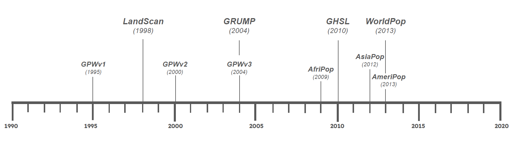
The need to fill the gap in population data availability led to the development of the first global gridded population dataset in the 1990s (see Figure 1): the Gridded Population of the World (GPW).1–3 By combining population counts from censuses at second-administrative levels (i.e. counties and districts) with spatially-explicit administrative boundary data, researchers created a raster dataset that depicts population counts at 5-minute grid resolution (roughly 10km at the equator) on a continuous surface of the earth.4 This data enabled researchers studying extreme weather (data that are commonly reported as a gridded surface) to incorporate population into their analyses without aggregating environmental data to subnational administrative units.
Since then, advancements in the technology used to collect remote sensing data, such as topography and land cover, have improved identification of urban areas.5 Increased computing power, improved spatial accuracy, and use of additional datasets such as night-time light satellite imagery, land cover, and digital elevation models (called ancillary data) have enabled researchers to advance the methods used to redistribute census population counts to grid cells at high resolution and accuracy.6 As a result, several gridded population datasets have been developed using different methods and input data, leading to datasets with varying spatial and population accuracy depending on the context. Below, we’ll highlight some of the similarities and differences between the prominent gridded population datasets that have been developed and identify appropriate use-case scenarios.
Common population density data sources
A comparison of the spatial resolution, temporal availability, data/methods used, and best use cases for each of the four datasets we’re highlighting in this post are summarized in Table 1 below, while Figure 1 (above) outlines the dates of first publication for each dataset. Without a proper understanding of how these data products are developed and their ideal use-cases, the research community is more likely to choose the wrong dataset for their project.7 In the subsequent sections, we introduce each dataset in additional detail.
Global Rural-Urban Mapping Project (GRUMP)
GRUMP is a series of global gridded population counts and densities created by Columbia University’s Centre for International Earth Science Information Network (CIESIN) in 2004, available for years 1990, 1995, and 2000.8 Using lightly-modeled dasymetric methods based on GPW population and NOAA night-time lights, it indicates the locations of urban settlements and delineates the spatial extents of urban areas at 30 arc-second (roughly 1 kilometer at the equator) resolution.6 In fact, it was the first global gridded population dataset to define urban areas and was widely used for two reasons:
- its urban footprint is based on stable-city lights which is an inclusive measure of urban areas
- the dichotomous definition of the urban footprint (urban or rural) is simple for researchers to use9
GRUMP’s popularity waned upon the creation of higher-resolution datasets that became available for more recent years, including the Global Human Settlement Layer (GHSL) created by the European Commission Joint Research Centre (JRC) in 2010.
Global Human Settlement Layer (GHSL)
Available in 5-year intervals from 1975 to 2020, GHSL data products are provided at a spatial resolution of 3 arc-seconds (roughly 100 meters at the equator). GHSL utilizes Landsat imagery (prior to 2014) and Sentinel-2 composite imagery (2014-forward) in an image classification method called Symbolic Machine Learning (SML) to map urban land cover and classify population and land area into seven classes along an urban-rural continuum.9,10
The GHSL population data product is made up of three datasets: GHS-POP (population size), GHS-BUILT (built-up areas), and GHS-SMOD (a Degree of Urbanization model grid that delineates settlement types using GHS-POP and GHS-BUILT).11
GHSL has been widely used to study the interactions between weather extremes, health, and populations. For example, Pinchoff and colleagues12 used GHS-BUILT to examine the impact of urbanicity on health in Tanzania. McGranahan and colleagues13 used GHS-SMOD to calculate urbanization rates in low-elevation coastal zones and estimate the effect of urbanization on weather extremes in deltaic regions. In another study, the authors examined spatial accessibility to healthcare in sub-Saharan Africa (SSA) using GHS-SMOD.14
LandScan
While it is a lower resolution data product, LandScan is another prominent global population distribution dataset that provides ambient (24-hour average) population distribution at 30 arc-seconds (roughly 1 kilometer at the equator) resolution, developed in 1998 by the Oak Ridge National Laboratory in Tennessee.15,16
In contrast to GRUMP and GHSL—which provide data at 5-year intervals—LandScan is available annually from 2000 through 2022. LandScan utilizes night-time light satellite imagery along with spatial information about elevation (Digital Elevation Models), slope (Digital Terrain Models), land cover, and populated place vector data within a multivariable dasymetric model that uses machine learning to assign the likelihood of population occurrence to each cell.
LandScan differs from other datasets in that it provides ambient population distribution, depicting not only where people sleep but where they travel, work, and socialize over a 24-hour period. While this may be an important distinction for some researchers, it sets the dataset apart from others, making it less comparable. Researchers should also take caution when comparing multiple versions of LandScan data—regular updates to the input data and distribution algorithm can cause comparability issues between versions.
WorldPop
WorldPop is another global gridded population distribution dataset that provides annual estimates from 2000 through 2020; however, WorldPop is provided at a higher resolution of 3 arc-seconds (roughly 100 meters at the equator). Developed by the University of Southampton in 2013, WorldPop uses Sentinel-1 and Sentinel-2 imagery in combination with spatial information on impervious surfaces (SRTM) and slope (DEM) in a dasymetric model with machine learning to estimate population distribution.17
WorldPop was created by combining three continental-scale population datasets:
- AfriPop (developed in 2009)
- AsiaPop (developed in 2012)
- AmeriPop (developed in 2013)
WorldPop’s population estimates are fractional (not integer), which can produce difficulties in interpretation since individual persons obviously cannot be divided up over an area. Its prediction model is good at estimating activity space with the caveat that it can overestimate population density in peri-urban areas while under-estimating population densities in urban centers.
| Metric | Global Urban-Rural Mapping Project (GRUMP) | Global Human Settlement Layer (GHSL) | LandScan | WorldPop |
|---|---|---|---|---|
| Spatial Resolution | 30 arc-seconds (~1 km) | 3 arc-seconds (~100m) | 30 arc-seconds (~1km) | 3 arc-seconds (~100m) |
| Temporal Availability | 1990, 1995, 2000 | 1975-2020 (5-year intervals) | 2000-2022 (annual) | 2000-2020 (annual) |
| Organization | CIESIN, Columbia University | European Commission | Oak Ridge National Laboratory | University of Southampton |
| Ancillary Data |
|
|
|
|
| Methods | Area-weighted reallocation | Dasymetric modeling with Symbolic Machine Learning (SML) is used to combine built-up areas (GHS-BUILT) and population size (GHS-POP) to create a settlement model (GHS-SMOD) based on Degree of Urbanization (DoU), which includes seven classes along an urban-rural continuum. | Dasymetric modeling with machine learning (ML). Likelihood of population occurrence in a particular cell is modeled based on probability coefficients, including roads (weighted by distance from cells to roads), slope (weighted by favorable slope categories), land cover (weighted by type and applying exclusions), and night-time lights (weighted by frequency). | Dasymetric modeling with machine learning (ML). A random forest prediction model is used to create a weight layer. |
| Advantages | The first of its kind, GRUMP was the ideal population distribution dataset used by researchers prior to 2010. | High resolution. Very accurate in areas with higher development. Not a dichotomous urban/rural variable, it allows re searchers to identify peri-urban areas. | Depicts ambient (24-hour average) population distribution, which captures not only where people sleep but where they travel, work, and socialize. Data available annually. | High resolution. Population density raster data allows researchers to define urban, peri-urban, and rural areas based on density percentages that are appropriate for that area. |
| Limitations | Data only available at 5-year intervals and not updated for recent years. Since it is based on proportional reallocation, it relies on accurate subnational population projections and a reliable nigh-time lights dataset. | Low degrees of accuracy in rural areas. Data only available at 5-year intervals. | Not comparable with other datasets due to its ambient nature. Regular updates to distribution algorithms makes it inadvisable to compare different versions of the dataset. | Population estimates are fractional (not integer), but people cannot exist over an entire area. Potential overestimates of population density in peri-urban areas and underestimates in urban centers. |
Comparing sources
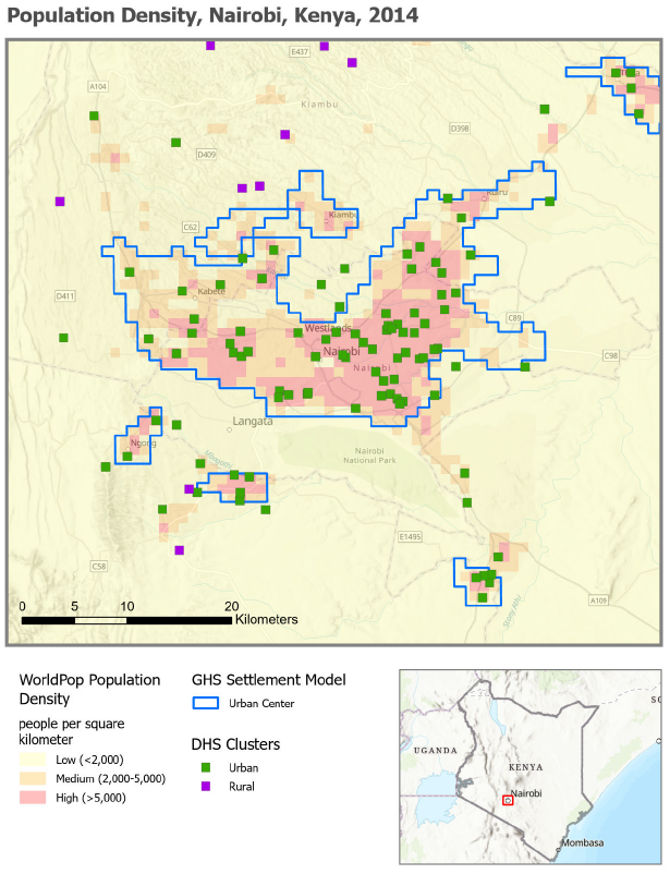
Representation of global population distribution is an increasingly important topic for researchers interested in human-environment interactions. It is vital that studies consider the advantages and limitations of the dataset they choose, as it has implications for statistical model outputs which can influence the conclusions drawn from their results. Researchers may benefit from downloading multiple datasets and comparing population density estimates based on each dataset for their study area. An example comparison is shown in Figure 2, a population density map of Nairobi, Kenya, depicting the spatial extent of the Nairobi urban center based on the GHS settlement model (GHS-SMOD) in an overlay with WorldPop population density. As the map shows, the spatial extent of the urban area is not in complete agreement between the two datasets.
In future posts, we’ll demonstrate methods to work with some of these datasets in R!
Getting Help
Questions or comments? Check out the IPUMS User Forum or reach out to IPUMS User Support at ipums@umn.edu.