On May 4th, PMA and IPUMS PMA co-hosted a Population Association of America 2021 virtual data workshop showcasing the new PMA contraceptive calendar data available for these samples:
- Burkina Faso 2020
- Congo (DR), Kinshasa 2019
- Congo (DR), Kongo Central 2019
- Kenya 2019
- Nigeria, Kano 2019
- Nigeria, Lagos 2019
These data represent contraceptive use, pregnancy, pregnancy termination, and birth information recalled by female respondents for each of several months preceding the PMA interview. Women sampled in Burkina Faso and Democratic Republic of the Congo were each asked to recall monthly information for up to 24 months, while women sampled from Kenya and Nigeria were asked to recall monthly information for up to 36 months. Their responses are recorded in a single comma delimited string, where information about each month is represented by one of the following codes:
- B = Birth
- P = Pregnant
- T = Pregnancy ended
- 0 = No family planning method used
- 1 = Female Sterilization
- 2 = Male Sterilization
- 3 = Implant
- 4 = IUD
- 5 = Injectables
- 7 = Pill
- 8 = Emergency Contraception
- 9 = Male Condom
- 10 = Female Condom
- 11 = Diaphragm
- 12 = Foam / Jelly
- 13 = Standard Days / Cycle beads
- 14 = LAM
- 30 = Rhythm method
- 31 = Withdrawal
- 39 = Other traditional methods
In this video, PMA and IPUMS PMA explain the background behind contraceptive calendar data and show some of the ways you might consider using it in longitudinal analysis. We also give a conceptual overview of the steps both R and Stata users should take to reshape the data into a long format. After the overview, R and Stata users split into separate breakout sessions to work with a hands-on coding example using data from the Kenya 2019 sample; this example shows how to build a Kaplan-Meier survival curve for cohorts of women who were using the same family planning method in the first month of the contraceptive calendar.
Breakout Session: R Users
R users can load a fixed-width IPUMS PMA data extract with help from the ipumsr package (if you’re new to this blog, check out detailed instructions here). We also use packages from tidyverse to reformat the data, as well as survival and ggfortify for specific survival analysis functions.
When you open any IPUMS PMA data extract from the Household and Female Survey, you’ll find the data organized with one respondent per row. Here, there are 9,549 rows each representing one female respondent (all other household members have been excluded):
dat
# A tibble: 9,549 × 17
         SAMPLE COUNTRY  YEAR HHID  PERSONID ELIGIBLE   EAID CONSENTFQ
      <int+lbl> <int+l> <int> <chr> <chr>    <int+lb>  <dbl> <int+lbl>
 1 40410 [Keny… 7 [Ken…  2019 4042… 4042019… 1 [Yes,… 4.04e8   1 [Yes]
 2 40410 [Keny… 7 [Ken…  2019 4042… 4042019… 1 [Yes,… 4.04e8   1 [Yes]
 3 40410 [Keny… 7 [Ken…  2019 4042… 4042019… 1 [Yes,… 4.04e8   1 [Yes]
 4 40410 [Keny… 7 [Ken…  2019 4042… 4042019… 1 [Yes,… 4.04e8   1 [Yes]
 5 40410 [Keny… 7 [Ken…  2019 4042… 4042019… 1 [Yes,… 4.04e8   1 [Yes]
 6 40410 [Keny… 7 [Ken…  2019 4042… 4042019… 1 [Yes,… 4.04e8   1 [Yes]
 7 40410 [Keny… 7 [Ken…  2019 4042… 4042019… 1 [Yes,… 4.04e8   1 [Yes]
 8 40410 [Keny… 7 [Ken…  2019 4042… 4042019… 1 [Yes,… 4.04e8   1 [Yes]
 9 40410 [Keny… 7 [Ken…  2019 4042… 4042019… 1 [Yes,… 4.04e8   1 [Yes]
10 40410 [Keny… 7 [Ken…  2019 4042… 4042019… 1 [Yes,… 4.04e8   1 [Yes]
11 40410 [Keny… 7 [Ken…  2019 4042… 4042019… 1 [Yes,… 4.04e8   1 [Yes]
12 40410 [Keny… 7 [Ken…  2019 4042… 4042019… 1 [Yes,… 4.04e8   1 [Yes]
13 40410 [Keny… 7 [Ken…  2019 4042… 4042019… 1 [Yes,… 4.04e8   1 [Yes]
14 40410 [Keny… 7 [Ken…  2019 4042… 4042019… 1 [Yes,… 4.04e8   1 [Yes]
15 40410 [Keny… 7 [Ken…  2019 4042… 4042019… 1 [Yes,… 4.04e8   1 [Yes]
16 40410 [Keny… 7 [Ken…  2019 4042… 4042019… 1 [Yes,… 4.04e8   1 [Yes]
17 40410 [Keny… 7 [Ken…  2019 4042… 4042019… 1 [Yes,… 4.04e8   1 [Yes]
18 40410 [Keny… 7 [Ken…  2019 4042… 4042019… 1 [Yes,… 4.04e8   1 [Yes]
19 40410 [Keny… 7 [Ken…  2019 4042… 4042019… 1 [Yes,… 4.04e8   1 [Yes]
20 40410 [Keny… 7 [Ken…  2019 4042… 4042019… 1 [Yes,… 4.04e8   1 [Yes]
# … with 9,529 more rows, and 9 more variables: FQINSTID <chr>,
#   CONSENTHQ <int+lbl>, FQWEIGHT <dbl>, STRATA <int+lbl>,
#   SUBNATIONAL <int+lbl>, AGE <int+lbl>, BIRTHEVENT <int+lbl>,
#   WORKYR <int+lbl>, CALENDARKE <chr+lbl>
For the purpose of this exercise only we create a short
identifying number for each respondent called ID. Then, we
select only the variables ID and CALENDARKE
(dropping all of the other variables pre-selected for every IPUMS PMA
extract).
dat <- dat %>%
  rowid_to_column("ID") %>%
  select(ID, CALENDARKE)

dat
# A tibble: 9,549 × 2
      ID CALENDARKE
   <int> <chr+lbl>
 1     1 0,0,B,P,P,P,P,P,P,P,P,0,0,0,0,0,0,0,0,0,0,0,0,3,3,3,3,3,3,3,…
 2     2 ,7,7,7,7,7,7,7,7,0,B,P,P,P,P,P,P,P,P,0,0,0,0,0,9,9,9,9,9,9,9…
 3     3 0,0,0,0,0,0,0,0,0,0,0,0,0,0,0,0,0,0,0,0,0,0,0,0,0,0,0,0,0,0,…
 4     4 0,0,0,0,0,0,0,0,0,0,0,0,0,0,0,0,0,0,0,0,0,0,0,0,0,0,0,0,0,0,…
 5     5 ,5,5,5,5,5,5,5,5,5,5,5,5,5,5,5,5,B,P,P,P,P,P,P,P,P,0,0,0,0,0…
 6     6 5,5,5,5,5,5,5,5,5,5,5,5,5,5,5,5,5,5,5,5,5,5,5,5,5,5,5,5,5,5,…
 7     7 5,5,5,5,5,5,0,0,0,0,0,0,0,0,0,0,0,0,0,0,0,0,0,0,B,P,P,P,P,P,…
 8     8 P,P,P,P,P,P,P,P,0,0,0,0,0,0,0,14,14,14,14,14,14,14,B,P,P,P,P…
 9     9 0,0,0,0,0,0,0,0,0,0,0,0,0,0,0,0,0,0,0,0,0,0,0,0,0,0,0,0,0,0,…
10    10 ,P,P,P,9,9,9,9,9,9,9,9,9,9,9,9,9,9,9,9,9,9,9,9,9,9,9,9,9,9,9…
11    11 ,0,0,0,0,0,0,0,0,0,0,0,0,0,0,0,0,0,0,0,0,0,0,0,0,0,0,0,0,0,0…
12    12 ,0,0,0,0,0,0,0,0,0,0,0,0,0,0,0,0,0,0,0,0,0,0,0,0,0,0,0,0,0,0…
13    13 ,P,P,P,P,P,P,P,9,9,9,9,9,9,9,9,9,9,9,9,9,9,9,9,9,9,9,9,9,9,9…
14    14 0,0,0,0,0,0,0,0,0,0,0,0,0,0,0,0,0,0,0,0,0,0,0,0,0,0,0,0,0,0,…
15    15 0,0,0,0,0,0,0,0,0,0,0,0,0,0,0,0,0,0,0,0,0,0,0,0,0,0,0,0,0,14…
16    16 3,3,3,3,3,3,3,3,3,3,3,3,3,3,3,3,3,3,3,3,3,3,3,3,3,3,3,3,3,3,…
17    17 ,5,5,5,5,5,5,5,5,5,5,5,5,5,5,5,5,5,5,5,5,5,5,5,5,5,5,5,5,5,5…
18    18 ,5,5,5,5,5,5,5,5,5,5,5,7,7,7,7,7,7,7,7,7,7,7,7,7,7,7,7,7,7,7…
19    19 0,0,0,0,0,0,9,0,0,0,0,0,0,0,0,0,0,0,0,0,0,0,0,0,0,0,0,0,0,0,…
20    20 ,P,P,P,P,P,P,P,5,5,5,5,5,0,0,0,0,0,0,0,0,0,0,0,0,0,0,0,0,0,0…
# … with 9,529 more rows
As you can see, CALENDARKE includes the response codes
shown above, each separated by a comma. Each string contains 36 codes:
these represent the 36 months from January 2017 through December 2019
(the last month in which Kenya 2019 samples were collected). The
left-most code represents the most recent available month.
Some strings begin with a comma (i.e. the most recent month is
blank). These are individuals who were interviewed in November 2019,
rather than December. When we split the string into 36 columns, we must
shift these individuals to the right, leaving a blank value in the
left-most column (December 2019). For example, notice the blank value
that appears in the new column cal_ke36 for the person
ID == 2.
# A tibble: 9,549 × 37
      ID cal_ke36 cal_ke35 cal_ke34 cal_ke33 cal_ke32 cal_ke31
   <int> <chr>    <chr>    <chr>    <chr>    <chr>    <chr>
 1     1 "0"      0        B        P        P        P
 2     2 ""       7        7        7        7        7
 3     3 "0"      0        0        0        0        0
 4     4 "0"      0        0        0        0        0
 5     5 ""       5        5        5        5        5
 6     6 "5"      5        5        5        5        5
 7     7 "5"      5        5        5        5        5
 8     8 "P"      P        P        P        P        P
 9     9 "0"      0        0        0        0        0
10    10 ""       P        P        P        9        9
11    11 ""       0        0        0        0        0
12    12 ""       0        0        0        0        0
13    13 ""       P        P        P        P        P
14    14 "0"      0        0        0        0        0
15    15 "0"      0        0        0        0        0
16    16 "3"      3        3        3        3        3
17    17 ""       5        5        5        5        5
18    18 ""       5        5        5        5        5
19    19 "0"      0        0        0        0        0
20    20 ""       P        P        P        P        P
# … with 9,529 more rows, and 30 more variables: cal_ke30 <chr>,
#   cal_ke29 <chr>, cal_ke28 <chr>, cal_ke27 <chr>, cal_ke26 <chr>,
#   cal_ke25 <chr>, cal_ke24 <chr>, cal_ke23 <chr>, cal_ke22 <chr>,
#   cal_ke21 <chr>, cal_ke20 <chr>, cal_ke19 <chr>, cal_ke18 <chr>,
#   cal_ke17 <chr>, cal_ke16 <chr>, cal_ke15 <chr>, cal_ke14 <chr>,
#   cal_ke13 <chr>, cal_ke12 <chr>, cal_ke11 <chr>, cal_ke10 <chr>,
#   cal_ke9 <chr>, cal_ke8 <chr>, cal_ke7 <chr>, cal_ke6 <chr>, …
Let’s now pivot the data from wide to long format so that we’ll be
able to mark time in a new column called MONTH.
The argument names_pattern pulls the number from each
variable starting with cal_ke, which we then put in the new
column MONTH.
options(tibble.print_min = 40)

dat <- dat %>%
  pivot_longer(
    starts_with("cal_ke"),
    names_pattern = "cal_ke(.*)",
    names_to = "MONTH",
    values_to = "FP"
  )

dat
# A tibble: 343,764 × 3
      ID MONTH FP
   <int> <chr> <chr>
 1     1 36    "0"
 2     1 35    "0"
 3     1 34    "B"
 4     1 33    "P"
 5     1 32    "P"
 6     1 31    "P"
 7     1 30    "P"
 8     1 29    "P"
 9     1 28    "P"
10     1 27    "P"
11     1 26    "P"
12     1 25    "0"
13     1 24    "0"
14     1 23    "0"
15     1 22    "0"
16     1 21    "0"
17     1 20    "0"
18     1 19    "0"
19     1 18    "0"
20     1 17    "0"
21     1 16    "0"
22     1 15    "0"
23     1 14    "0"
24     1 13    "3"
25     1 12    "3"
26     1 11    "3"
27     1 10    "3"
28     1 9     "3"
29     1 8     "3"
30     1 7     "3"
31     1 6     "3"
32     1 5     "3"
33     1 4     "3"
34     1 3     "3"
35     1 2     "3"
36     1 1     "3"
37     2 36    ""
38     2 35    "7"
39     2 34    "7"
40     2 33    "7"
# … with 343,724 more rowsWe’ve now created a variable FP containing the original
CALENDARKE variable codes. This variable will be much
easier to work with if we 1) convert it into a factor, and 2) replace
missing values with NA (e.g. month 36 for individuals
interviewed in November 2018). We’ll also coerce MONTH from
a “character” to an “integer” class.
dat <- dat %>%
  mutate(
    MONTH = as.integer(MONTH),
    FP = FP %>%
      na_if("") %>%
      fct_recode(
        "Birth" = "B",
        "Pregnant" = "P",
        "Pregnancy ended" = "T",
        "No family planning method used" = "0",
        "Female Sterilization" = "1",
        "Male Sterilization" = "2",
        "Implant" = "3",
        "IUD" = "4",
        "Injectables" = "5",
        "Pill" = "7",
        "Emergency Contraception" = "8",
        "Male Condom" = "9",
        "Female Condom" = "10",
        "Diaphragm" = "11",
        "Foam / Jelly" = "12",
        "Standard Days / Cycle beads" = "13",
        "LAM" = "14",
        "Rhythm method" = "30",
        "Withdrawal" = "31",
        "Other traditional methods" = "39"
      )
  )

dat
# A tibble: 343,764 × 3
      ID MONTH FP
   <int> <int> <fct>
 1     1    36 No family planning method used
 2     1    35 No family planning method used
 3     1    34 Birth
 4     1    33 Pregnant
 5     1    32 Pregnant
 6     1    31 Pregnant
 7     1    30 Pregnant
 8     1    29 Pregnant
 9     1    28 Pregnant
10     1    27 Pregnant
11     1    26 Pregnant
12     1    25 No family planning method used
13     1    24 No family planning method used
14     1    23 No family planning method used
15     1    22 No family planning method used
16     1    21 No family planning method used
17     1    20 No family planning method used
18     1    19 No family planning method used
19     1    18 No family planning method used
20     1    17 No family planning method used
21     1    16 No family planning method used
22     1    15 No family planning method used
23     1    14 No family planning method used
24     1    13 Implant
25     1    12 Implant
26     1    11 Implant
27     1    10 Implant
28     1     9 Implant
29     1     8 Implant
30     1     7 Implant
31     1     6 Implant
32     1     5 Implant
33     1     4 Implant
34     1     3 Implant
35     1     2 Implant
36     1     1 Implant
37     2    36 <NA>
38     2    35 Pill
39     2    34 Pill
40     2    33 Pill
# … with 343,724 more rows
We’re now ready to begin our analysis. To keep our example simple, our survival curves will show the duration of continuously used family planning methods for cohorts of women who were using the same method in January 2017. These survival curves will estimate the probability that an individual “survives” - or continues using - a given method at each of 36 months, assuming that she used it in month 1. We’ll exclude the duration of use after any break (for example, if a woman stopped using family planning to become pregnant, but then started again afterward).
Let’s begin with women who were using the contraceptive pill in
January 2017. Remove all other women, saving those who remain as a
sub-sample called pills:
pills <- dat %>%
  group_by(ID) %>%
  mutate(use_m1 = case_when(FP == "Pill" & MONTH == 1 ~ TRUE) %>% any()) %>%
  filter(use_m1)

pills
# A tibble: 10,332 × 4
# Groups:   ID [287]
      ID MONTH FP          use_m1
   <int> <int> <fct>       <lgl>
 1    18    36 <NA>        TRUE
 2    18    35 Injectables TRUE
 3    18    34 Injectables TRUE
 4    18    33 Injectables TRUE
 5    18    32 Injectables TRUE
 6    18    31 Injectables TRUE
 7    18    30 Injectables TRUE
 8    18    29 Injectables TRUE
 9    18    28 Injectables TRUE
10    18    27 Injectables TRUE
11    18    26 Injectables TRUE
12    18    25 Injectables TRUE
13    18    24 Pill        TRUE
14    18    23 Pill        TRUE
15    18    22 Pill        TRUE
16    18    21 Pill        TRUE
17    18    20 Pill        TRUE
18    18    19 Pill        TRUE
19    18    18 Pill        TRUE
20    18    17 Pill        TRUE
21    18    16 Pill        TRUE
22    18    15 Pill        TRUE
23    18    14 Pill        TRUE
24    18    13 Pill        TRUE
25    18    12 Pill        TRUE
26    18    11 Pill        TRUE
27    18    10 Pill        TRUE
28    18     9 Pill        TRUE
29    18     8 Pill        TRUE
30    18     7 Pill        TRUE
31    18     6 Pill        TRUE
32    18     5 Pill        TRUE
33    18     4 Pill        TRUE
34    18     3 Pill        TRUE
35    18     2 Pill        TRUE
36    18     1 Pill        TRUE
37    39    36 Pill        TRUE
38    39    35 Pill        TRUE
39    39    34 Pill        TRUE
40    39    33 Pill        TRUE
# … with 10,292 more rows
The next several steps will help us remove every record for each woman except for the last recorded month in which she used the pill. For those whose last month is month 36, we will say she “survived” the full observation period.
To avoid re-entry cases (returning to use of the pill), we’ll find
the earliest month that a woman in this cohort was not using
the pill. The month prior to this will be her last_month of
using the pill. For the first person in this cohort
ID == 18, for example, the last_month of use
should be MONTH == 24.
pills <- pills %>%
  mutate(
    non_use_month = case_when(FP != "Pill" | is.na(FP) ~ MONTH),
    last_month = ifelse(
      all(is.na(non_use_month)),
      36,
      min(non_use_month, na.rm = T) - 1
    )
  )

pills
# A tibble: 10,332 × 6
# Groups:   ID [287]
      ID MONTH FP          use_m1 non_use_month last_month
   <int> <int> <fct>       <lgl>          <int>      <dbl>
 1    18    36 <NA>        TRUE              36         24
 2    18    35 Injectables TRUE              35         24
 3    18    34 Injectables TRUE              34         24
 4    18    33 Injectables TRUE              33         24
 5    18    32 Injectables TRUE              32         24
 6    18    31 Injectables TRUE              31         24
 7    18    30 Injectables TRUE              30         24
 8    18    29 Injectables TRUE              29         24
 9    18    28 Injectables TRUE              28         24
10    18    27 Injectables TRUE              27         24
11    18    26 Injectables TRUE              26         24
12    18    25 Injectables TRUE              25         24
13    18    24 Pill        TRUE              NA         24
14    18    23 Pill        TRUE              NA         24
15    18    22 Pill        TRUE              NA         24
16    18    21 Pill        TRUE              NA         24
17    18    20 Pill        TRUE              NA         24
18    18    19 Pill        TRUE              NA         24
19    18    18 Pill        TRUE              NA         24
20    18    17 Pill        TRUE              NA         24
21    18    16 Pill        TRUE              NA         24
22    18    15 Pill        TRUE              NA         24
23    18    14 Pill        TRUE              NA         24
24    18    13 Pill        TRUE              NA         24
25    18    12 Pill        TRUE              NA         24
26    18    11 Pill        TRUE              NA         24
27    18    10 Pill        TRUE              NA         24
28    18     9 Pill        TRUE              NA         24
29    18     8 Pill        TRUE              NA         24
30    18     7 Pill        TRUE              NA         24
31    18     6 Pill        TRUE              NA         24
32    18     5 Pill        TRUE              NA         24
33    18     4 Pill        TRUE              NA         24
34    18     3 Pill        TRUE              NA         24
35    18     2 Pill        TRUE              NA         24
36    18     1 Pill        TRUE              NA         24
37    39    36 Pill        TRUE              NA         36
38    39    35 Pill        TRUE              NA         36
39    39    34 Pill        TRUE              NA         36
40    39    33 Pill        TRUE              NA         36
# … with 10,292 more rows
We must now identify whether the last_month represents
cessation or right-censoring. Remember that a large number of women in
our sample have missing values in the 36th month: they are
right-censored at month 35 if they had been continuously using
the pill until that time, so we cannot say that they ceased using at
month 35!
To make this easier, we’ll create a logical variable
right_censored that simply indicates whether each person is
missing a value for MONTH == 36.
# A tibble: 10,332 × 7
# Groups:   ID [287]
      ID MONTH FP       use_m1 non_use_month last_month right_censored
   <int> <int> <fct>    <lgl>          <int>      <dbl> <lgl>
 1    18    36 <NA>     TRUE              36         24 TRUE
 2    18    35 Injecta… TRUE              35         24 TRUE
 3    18    34 Injecta… TRUE              34         24 TRUE
 4    18    33 Injecta… TRUE              33         24 TRUE
 5    18    32 Injecta… TRUE              32         24 TRUE
 6    18    31 Injecta… TRUE              31         24 TRUE
 7    18    30 Injecta… TRUE              30         24 TRUE
 8    18    29 Injecta… TRUE              29         24 TRUE
 9    18    28 Injecta… TRUE              28         24 TRUE
10    18    27 Injecta… TRUE              27         24 TRUE
11    18    26 Injecta… TRUE              26         24 TRUE
12    18    25 Injecta… TRUE              25         24 TRUE
13    18    24 Pill     TRUE              NA         24 TRUE
14    18    23 Pill     TRUE              NA         24 TRUE
15    18    22 Pill     TRUE              NA         24 TRUE
16    18    21 Pill     TRUE              NA         24 TRUE
17    18    20 Pill     TRUE              NA         24 TRUE
18    18    19 Pill     TRUE              NA         24 TRUE
19    18    18 Pill     TRUE              NA         24 TRUE
20    18    17 Pill     TRUE              NA         24 TRUE
21    18    16 Pill     TRUE              NA         24 TRUE
22    18    15 Pill     TRUE              NA         24 TRUE
23    18    14 Pill     TRUE              NA         24 TRUE
24    18    13 Pill     TRUE              NA         24 TRUE
25    18    12 Pill     TRUE              NA         24 TRUE
26    18    11 Pill     TRUE              NA         24 TRUE
27    18    10 Pill     TRUE              NA         24 TRUE
28    18     9 Pill     TRUE              NA         24 TRUE
29    18     8 Pill     TRUE              NA         24 TRUE
30    18     7 Pill     TRUE              NA         24 TRUE
31    18     6 Pill     TRUE              NA         24 TRUE
32    18     5 Pill     TRUE              NA         24 TRUE
33    18     4 Pill     TRUE              NA         24 TRUE
34    18     3 Pill     TRUE              NA         24 TRUE
35    18     2 Pill     TRUE              NA         24 TRUE
36    18     1 Pill     TRUE              NA         24 TRUE
37    39    36 Pill     TRUE              NA         36 FALSE
38    39    35 Pill     TRUE              NA         36 FALSE
39    39    34 Pill     TRUE              NA         36 FALSE
40    39    33 Pill     TRUE              NA         36 FALSE
# … with 10,292 more rows
We’ll create another logical variable ceased to indicate
whether each woman actually stopped using the pill at her
last_month. If not (either because last_month
is 36, or she is right-censored and last_month is 35), it
will take the value FALSE.
pills <- pills %>%
  mutate(
    ceased = case_when(
      right_censored & last_month == 35 ~ F,
      last_month == 36 ~ F,
      last_month < 36 ~ T
    )
  ) %>%
  select(ID, MONTH, FP, last_month, ceased)

pills
# A tibble: 10,332 × 5
# Groups:   ID [287]
      ID MONTH FP          last_month ceased
   <int> <int> <fct>            <dbl> <lgl>
 1    18    36 <NA>                24 TRUE
 2    18    35 Injectables         24 TRUE
 3    18    34 Injectables         24 TRUE
 4    18    33 Injectables         24 TRUE
 5    18    32 Injectables         24 TRUE
 6    18    31 Injectables         24 TRUE
 7    18    30 Injectables         24 TRUE
 8    18    29 Injectables         24 TRUE
 9    18    28 Injectables         24 TRUE
10    18    27 Injectables         24 TRUE
11    18    26 Injectables         24 TRUE
12    18    25 Injectables         24 TRUE
13    18    24 Pill                24 TRUE
14    18    23 Pill                24 TRUE
15    18    22 Pill                24 TRUE
16    18    21 Pill                24 TRUE
17    18    20 Pill                24 TRUE
18    18    19 Pill                24 TRUE
19    18    18 Pill                24 TRUE
20    18    17 Pill                24 TRUE
21    18    16 Pill                24 TRUE
22    18    15 Pill                24 TRUE
23    18    14 Pill                24 TRUE
24    18    13 Pill                24 TRUE
25    18    12 Pill                24 TRUE
26    18    11 Pill                24 TRUE
27    18    10 Pill                24 TRUE
28    18     9 Pill                24 TRUE
29    18     8 Pill                24 TRUE
30    18     7 Pill                24 TRUE
31    18     6 Pill                24 TRUE
32    18     5 Pill                24 TRUE
33    18     4 Pill                24 TRUE
34    18     3 Pill                24 TRUE
35    18     2 Pill                24 TRUE
36    18     1 Pill                24 TRUE
37    39    36 Pill                36 FALSE
38    39    35 Pill                36 FALSE
39    39    34 Pill                36 FALSE
40    39    33 Pill                36 FALSE
# … with 10,292 more rowsRemove all rows except for the row containing each woman’s
last_month. The result will be a data frame where each
woman in the pills cohort occupies only one row,
which 1) shows her last month of recorded use and 2) indicates whether
we know that she actually stopped using the pill in her last month.
# A tibble: 287 × 5
# Groups:   ID [287]
      ID MONTH FP    last_month ceased
   <int> <int> <fct>      <dbl> <lgl>
 1    18    24 Pill          24 TRUE
 2    39    36 Pill          36 FALSE
 3    44     5 Pill           5 TRUE
 4    59    36 Pill          36 FALSE
 5    60     6 Pill           6 TRUE
 6    99    36 Pill          36 FALSE
 7   188    36 Pill          36 FALSE
 8   202    36 Pill          36 FALSE
 9   218    35 Pill          35 FALSE
10   233    12 Pill          12 TRUE
11   260     2 Pill           2 TRUE
12   290    35 Pill          35 FALSE
13   298    20 Pill          20 TRUE
14   335    12 Pill          12 TRUE
15   340    11 Pill          11 TRUE
16   419    36 Pill          36 FALSE
17   423    36 Pill          36 FALSE
18   428     4 Pill           4 TRUE
19   460    16 Pill          16 TRUE
20   488    17 Pill          17 TRUE
21   551    32 Pill          32 TRUE
22   669    36 Pill          36 FALSE
23   697    23 Pill          23 TRUE
24   707    26 Pill          26 TRUE
25   757    33 Pill          33 TRUE
26   767    23 Pill          23 TRUE
27   785    18 Pill          18 TRUE
28   836     1 Pill           1 TRUE
29   837    12 Pill          12 TRUE
30   850    35 Pill          35 FALSE
31   930    36 Pill          36 FALSE
32   943    13 Pill          13 TRUE
33   955     5 Pill           5 TRUE
34   977    36 Pill          36 FALSE
35  1001    36 Pill          36 FALSE
36  1037    36 Pill          36 FALSE
37  1120     7 Pill           7 TRUE
38  1167    19 Pill          19 TRUE
39  1233    36 Pill          36 FALSE
40  1271    32 Pill          32 TRUE
# … with 247 more rows
Let’s now fit the Kaplan Meier estimator with survfit,
which takes a survival object created by Surv. The function
summary shows the survival probabilities at each month in a
column called survival:
Call: survfit(formula = Surv(last_month, ceased) ~ 1, data = pills)
time n.risk n.event survival std.err lower 95% CI upper 95% CI
1 287 4 0.986 0.00692 0.973 1.000
2 283 6 0.965 0.01082 0.944 0.987
3 277 7 0.941 0.01393 0.914 0.968
4 270 10 0.906 0.01723 0.873 0.940
5 260 14 0.857 0.02066 0.818 0.899
6 246 4 0.843 0.02146 0.802 0.886
7 242 7 0.819 0.02274 0.775 0.865
8 235 5 0.801 0.02355 0.757 0.849
9 230 3 0.791 0.02400 0.745 0.839
10 227 5 0.774 0.02471 0.727 0.823
11 222 8 0.746 0.02571 0.697 0.798
12 214 21 0.672 0.02770 0.620 0.729
13 193 9 0.641 0.02831 0.588 0.699
14 184 6 0.620 0.02865 0.567 0.679
15 178 2 0.613 0.02875 0.559 0.672
16 176 5 0.596 0.02897 0.542 0.655
17 171 8 0.568 0.02924 0.513 0.628
18 163 6 0.547 0.02938 0.492 0.608
19 157 7 0.523 0.02948 0.468 0.584
20 150 2 0.516 0.02950 0.461 0.577
21 148 2 0.509 0.02951 0.454 0.570
22 146 3 0.498 0.02951 0.444 0.560
23 143 6 0.477 0.02948 0.423 0.539
24 137 9 0.446 0.02934 0.392 0.507
25 128 3 0.436 0.02927 0.382 0.497
26 125 4 0.422 0.02915 0.368 0.483
27 121 1 0.418 0.02912 0.365 0.479
28 120 3 0.408 0.02901 0.355 0.469
29 117 2 0.401 0.02893 0.348 0.462
31 115 2 0.394 0.02884 0.341 0.455
32 113 3 0.383 0.02870 0.331 0.444
33 110 3 0.373 0.02854 0.321 0.433
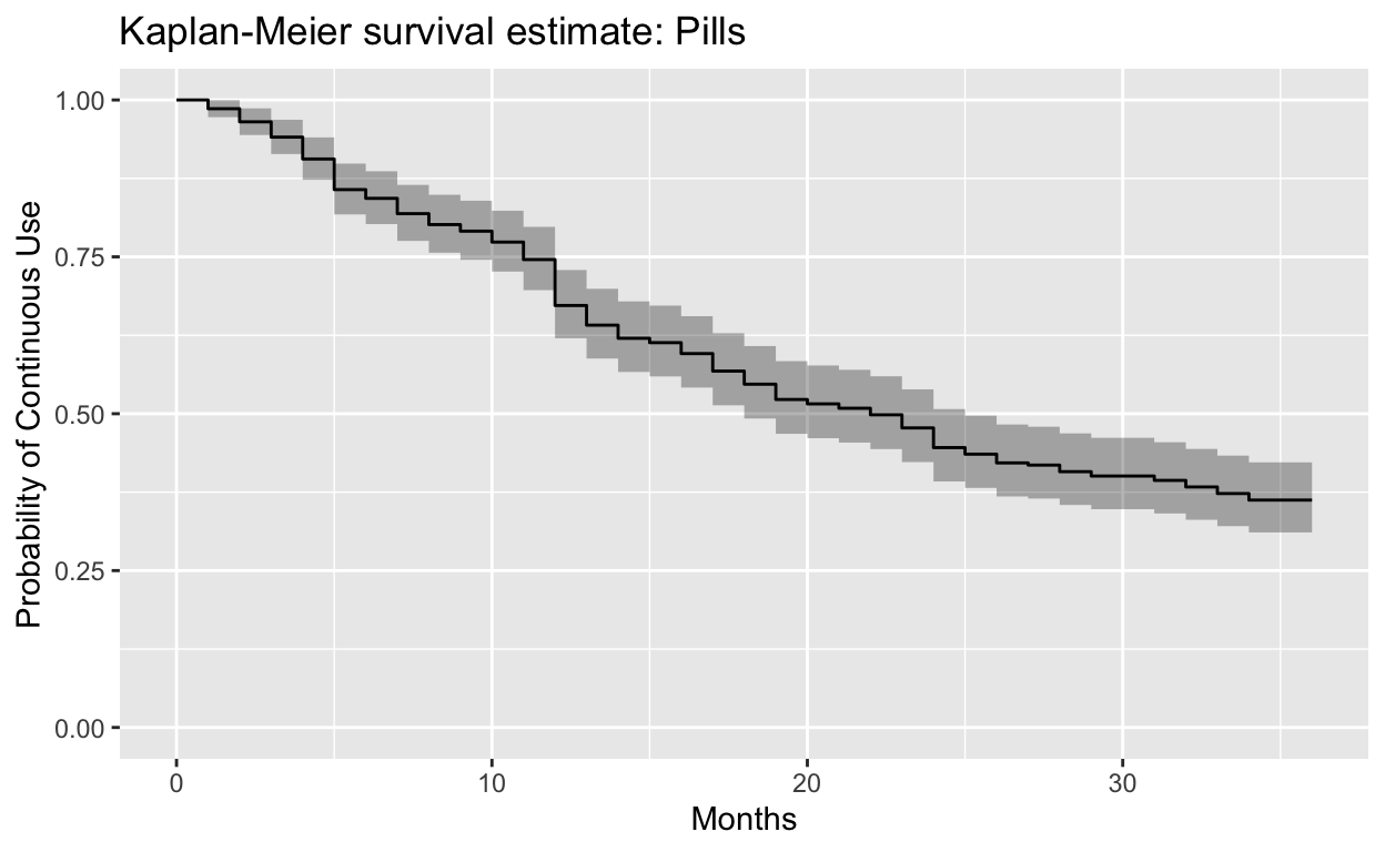
34 107 3 0.362 0.02837 0.311 0.422We can plot this with autoplot:
autoplot(
  pills,
  main = "Kaplan-Meier survival estimate: Pills",
  xlab = "Months",
  ylab = "Probability of Continuous Use",
  ylim = c(0, 1),
  censor = F
)
For additional examples using other family planning methods, download the R Markdown script from this breakout session. Video from the session is included below:
Breakout Session: Stata Users
IPUMS PMA extracts for Stata should be decompressed before use and loaded with an appropriate filepath:
. clear
. use "[filepath]/pma_00001.dta"
. cd "[filepath]"
. set more offAs shown in the R example above, this dataset contains 9,549 rows
where each row represents one respondent to the Female Questionnaire.
You’ll find a unique identification number for each respondent in
personid, and their comma-separated contraceptive calendar
strings in calendarke. We’ll show these two variables for
the first 3 respondents:
. list personid calendarke in 1/3

     +----------------------------------------------------------------------+
  1. |                                           personid                   |
     |                              404201900050442019002                   |
     |----------------------------------------------------------------------|
     | calendarke                                                           |
     |   0,0,B,P,P,P,P,P,P,P,P,0,0,0,0,0,0,0,0,0,0,0,0,3,3,3,3,3,3,3,3,3,.. |
     +----------------------------------------------------------------------+

     +----------------------------------------------------------------------+
  2. |                                           personid                   |
     |                              404201900009272019002                   |
     |----------------------------------------------------------------------|
     | calendarke                                                           |
     |   ,7,7,7,7,7,7,7,7,0,B,P,P,P,P,P,P,P,P,0,0,0,0,0,9,9,9,9,9,9,9,9,9.. |
     +----------------------------------------------------------------------+

     +----------------------------------------------------------------------+
  3. |                                           personid                   |
     |                              404201900099612019003                   |
     |----------------------------------------------------------------------|
     | calendarke                                                           |
     |   0,0,0,0,0,0,0,0,0,0,0,0,0,0,0,0,0,0,0,0,0,0,0,0,0,0,0,0,0,0,0,0,.. |
     +----------------------------------------------------------------------+
As you can see, calendarke includes the same
contraceptive calendar codes shown above, each separated by a comma.
Each string contains 36 codes: these represent the 36 months from
January 2017 through December 2019 (the last month in which Kenya 2019
samples were collected). The left-most code represents the most
recent available month.
Notice the second listed person
(personid 404201900009272019002); their
calendarke string begins with a comma rather than a
response code. This indicates a person who was interviewed in November
2019, rather than December. Because December 2019 would have been a
future month for such a person, their first value is blank.
Split the calendarke string into 36 separate columns
with the split function:
. split calendarke, p(,) gen(cal_ke)
variables created as string:
cal_ke1   cal_ke7   cal_ke13  cal_ke19  cal_ke25  cal_ke31
cal_ke2   cal_ke8   cal_ke14  cal_ke20  cal_ke26  cal_ke32
cal_ke3   cal_ke9   cal_ke15  cal_ke21  cal_ke27  cal_ke33
cal_ke4   cal_ke10  cal_ke16  cal_ke22  cal_ke28  cal_ke34
cal_ke5   cal_ke11  cal_ke17  cal_ke23  cal_ke29  cal_ke35
cal_ke6   cal_ke12  cal_ke18  cal_ke24  cal_ke30  cal_ke36
Then, reshape the data from wide to long format as shown in the R
example above. The index number for each month will pivot downward into
a new column called month, and the woman’s response code
for each month will pivot downward into an adjacent column called
cal_ke:
. reshape long cal_ke, i(personid) j(month)
(note: j = 1 2 3 4 5 6 7 8 9 10 11 12 13 14 15 16 17 18 19 20 21 22 23 24 25
> 26 27 28 29 30 31 32 33 34 35 36)

Data                               wide   ->   long
-----------------------------------------------------------------------------
Number of obs.                     9549   ->  343764
Number of variables                  52   ->      18
j variable (36 values)                    ->   month
xij variables:
           cal_ke1 cal_ke2 ... cal_ke36   ->   cal_ke
-----------------------------------------------------------------------------
Notice that the dataset now has 343,764 rows, where each of our 9,549
respondents occupies 36 rows apiece (one for each
month).
By default, Stata numbered each month in increasing order from left
to right. As we’ve discussed, however, the contraceptive calendar data
are chronologically organized from right to left (the most recent month
is stored in the first month of the calendarke string). We
suggest renumbering the cal_ke variables here so that
cal_ke1 represents the first month, January 2017.
. replace month = 37 - month
(343,764 real changes made)
. sort personid month
You might also find it useful to create century month codes
cmc for each month, beginning with 1405 for January
2017.
. gen cmc = month + 1404As a final clean-up step, we create a numeric version of
cal_ke called numcal_ke by changing the codes
for pregnancy, pregnancy termination, and birth to 90,
91, and 92 respectively. We then provide
labels to each of the values in numcal_ke.
. gen numcal_ke = cal_ke
(3,755 missing values generated)
. replace numcal_ke = "90" if numcal_ke == "P"
(24,364 real changes made)
. replace numcal_ke = "91" if numcal_ke == "T"
(341 real changes made)
. replace numcal_ke = "92" if numcal_ke == "B"
(2,934 real changes made)
. destring numcal_ke, replace
numcal_ke: all characters numeric; replaced as byte
(3755 missing values generated)

. label define calendar 92 "Birth" 90 "Pregnant" 91 "Pregnancy ended" 0 "No
> family planning method used" 1 "Female Sterilization" 2 "Male Sterilization" 3
> "Implant" 4 "IUD" 5 "Injectables" 7 "Pill" 8 "Emergency Contraception" 9 "Male
> Condom" 10 "Female Condom" 11 "Diaphragm" 12 "Foam / Jelly" 13 "Standard Days /
> Cycle beads" 14 "LAM" 30 "Rhythm method" 31 "Withdrawal" 39 "Other traditional
> methods"

. label values numcal_ke calendar
Finally, we’re ready to begin our analysis. As with the R example above, we’ll create survival curves showing the duration of continuously used family planning methods for cohorts of women who were using the same method in January 2017. These curves will estimate the probability that an individual “survives” - or continues using - a given method at each of 36 months, assuming that she used it in month 1. We’ll exclude the duration of use after any break (for example, if a woman stopped using family planning to become pregnant, but then started again afterward).
Consider the cohort of women who were all using the contraceptive
pill in January 2017 (month 1). We’ll flag these cases and include all
rows from those women in a sub-sample called
pill_sample:
. recode numcal_ke (7=1) (else=0), gen(pill)
(162306 differences between numcal_ke and pill)
. gen pill_temp = 0
. replace pill_temp = 1 if pill == 1 & month == 1
(287 real changes made)
. egen pill_sample = max(pill_temp), by(personid)
The function stset establishes the data in memory as
“survival-time” data, where the variable month records time
in months, the identification number for each person is provided by
id(personid), and cessation of use
(i.e. failure) is marked by the first instance where
pill==0 for each person in the sub-sample.
. stset month, id(personid) failure(pill==0)

                id:  personid
     failure event:  pill == 0
obs. time interval:  (month[_n-1], month]
 exit on or before:  failure

-----------------------------------------------------------------------------
> -
    343,764  total observations
    328,001  observations begin on or after (first) failure
-----------------------------------------------------------------------------
> -
     15,763  observations remaining, representing
      9,549  subjects
      9,463  failures in single-failure-per-subject data
     15,763  total analysis time at risk and under observation
                                                at risk from t =         0
                                     earliest observed entry t =         0
                                          last observed exit t =        36
The function sts list produces a similar table to the
one produced by summary(pills) in the R example above. The
column Survivor Function estimates the probability of
“surviving” - or continuously using - the pill at each month shown in
the column Time.
.  sts list if pill_sample == 1

         failure _d:  pill == 0
   analysis time _t:  month
                 id:  personid

           Beg.          Net            Survivor      Std.
  Time    Total   Fail   Lost           Function     Error     [95% Conf. Int.]
-------------------------------------------------------------------------------
     2      287      4      0             0.9861    0.0069     0.9633    0.9947
     3      283      6      0             0.9652    0.0108     0.9362    0.9811
     4      277      7      0             0.9408    0.0139     0.9064    0.9628
     5      270     10      0             0.9059    0.0172     0.8658    0.9345
     6      260     14      0             0.8571    0.0207     0.8111    0.8927
     7      246      4      0             0.8432    0.0215     0.7957    0.8805
     8      242      7      0             0.8188    0.0227     0.7692    0.8588
     9      235      5      0             0.8014    0.0235     0.7504    0.8431
    10      230      3      0             0.7909    0.0240     0.7392    0.8336
    11      227      5      0             0.7735    0.0247     0.7206    0.8177
    12      222      8      0             0.7456    0.0257     0.6911    0.7920
    13      214     21      0             0.6725    0.0277     0.6149    0.7234
    14      193      9      0             0.6411    0.0283     0.5827    0.6936
    15      184      6      0             0.6202    0.0286     0.5614    0.6735
    16      178      2      0             0.6132    0.0287     0.5543    0.6668
    17      176      5      0             0.5958    0.0290     0.5366    0.6500
    18      171      8      0             0.5679    0.0292     0.5085    0.6229
    19      163      6      0             0.5470    0.0294     0.4876    0.6025
    20      157      7      0             0.5226    0.0295     0.4633    0.5786
    21      150      2      0             0.5157    0.0295     0.4564    0.5717
    22      148      2      0             0.5087    0.0295     0.4495    0.5648
    23      146      3      0             0.4983    0.0295     0.4391    0.5545
    24      143      6      0             0.4774    0.0295     0.4185    0.5337
    25      137      9      0             0.4460    0.0293     0.3878    0.5024
    26      128      3      0             0.4355    0.0293     0.3776    0.4920
    27      125      4      0             0.4216    0.0291     0.3641    0.4779
    28      121      1      0             0.4181    0.0291     0.3607    0.4744
    29      120      3      0             0.4077    0.0290     0.3506    0.4639
    30      117      2      0             0.4007    0.0289     0.3438    0.4568
    32      115      2      0             0.3937    0.0288     0.3371    0.4498
    33      113      3      0             0.3833    0.0287     0.3271    0.4391
    34      110      3      0             0.3728    0.0285     0.3170    0.4285
    35      107      3      0             0.3624    0.0284     0.3070    0.4178
    36      104     18     86             0.2997    0.0270     0.2477    0.3532
-------------------------------------------------------------------------------
A survival curve representing this table can be made with:
sts graph if pill_sample == 1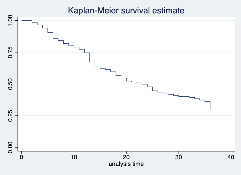
For additional examples using other family planning methods, download the Stata .do file from this breakout session here. Video from the session is included below:
Download Links
- Powerpoint Slides
- R Markdown Script
- Stata .do File
- Chat Transcript (participant names are redacted)