Automated Analysis of a Data Workflow - Part 2

In part 1 we discussed how Pandas and Bokeh work to find and highlight potential concerns in the data our researchers are producing across a broad range of samples and variables. In today’s part 2, we tackle the role of Jupyter in pulling all of these insights into a static, easily shared report and a reusable notebook that can be used to explore any issues identified by our tool. Finally, we’ll discuss how Anaconda is used to package the tool and isolate its dependencies from other Python tools we provide.

Jupyter

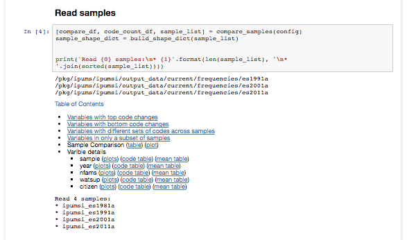
The generated report includes a lot of useful information about variables in the analyzed samples, including:

• Variables that appear in only a subset of samples
• Variables that have varying sets of codes across samples
• A full plot on the maximal frequency change for a code for each variable
• A user-configurable number of detailed plots for the variables showing the greatest change across samples.

The bulk of the code is in a Python module to do the analysis and generate the plots. We import this in a template notebook that breaks the analysis into sections and provides a table of contents. Our researchers execute a wrapper script that uses command-line configuration options to configure the report to be generated. This configuration is also stored as an .ini file which the users can edit to refine subsequent generations of the report, so the wrapper script can also take in this .ini file in lieu of command-line configuration options.

This .ini configuration file is injected into an in-memory version of the Jupyter notebook that is executed using the nbconvert library. This allows us to emit a static HTML report for easy redistribution via e-mail or the shared file system. We have users of varying degrees of technical inclination and toleration, so static HTML output requires the least effort and technical expertise to review. The following code shows the basic outline of turning a template notebook into a static HTML report.

file_writer = FilesWriter()
with open(nb_file) as f:
     nb = nbformat.read(f, as_version=4)
nb.cells[1]['source'] = '\n'.join([nb.cells[1]['source'], 'config_file=\'{}\''.format(config_file)])
(output, resources) = nb_exporter.from_notebook_node(nb)
ep.preprocess(nb, {'metadata': {'path': exe_path}})
cssp = CSSHTMLHeaderPreprocessor()
(nb, resources) = cssp.preprocess(nb, {'metadata': {'path': reports_dir}, 'config_dir': reports_dir})
html_exporter = HTMLExporter()
html_exporter.template_file = 'full'

This handles the majority of user needs. The configuration can be altered and the report regenerated as often as is necessary, allowing researchers to iterate over the data processing workflow and check their work and changes quickly. However, this workflow can be a bit clunky, especially for our more technologically-inclined users who are already exploring Jupyter notebooks for their own purposes.

For instance, what happens when a variable of interest is not one of the configured range of variables that are fully analyzed in the default report? We mentioned before that most of the code to generate the report is packaged as a library imported into the notebook, so the researcher already has access to example code for generating the plots and tables for a given variable right there within the notebook. With access to the .ipynb notebook file, a technically savvy researcher could simply duplicate a notebook cell and alter it to display the variable they care about. So, a few more lines of code are used to emit an .ipynb notebook file next to the static HTML report.

(output, resources) = html_exporter.from_notebook_node(nb)
file_writer.write(output, resources, os.path.join(reports_dir, nb_name))

We have a few general purpose computing servers available with JupyterHub installed, and users are able to put our generated analysis reports in their network home directory, which is accessible on these servers. We inject a link into the static report which goes to the notebook on one of these general purpose JupyterHubs. This allows the users to edit the .ipynb notebook and add more plots for specific variables of interest identified in the overview sections, and they can do this without having to alter the configuration and re-run the report from the command line. Researchers could also fix identified errors, re-run affected datasets in the background, and re-run the analysis report all from within Jupyter to see whether the fixes worked as intended. This creates a powerful new way of iteratively working through the data pipeline over and over again without ever leaving the Jupyter notebook environment.

We also have other Python libraries for interogating the dataset metadata. Users can use these libraries to investigate metadata issues that crop up in the analysis, and again they can do this from directly within the report itself. One common action will be to examine the expected “universe”, or expected range of results for a variable across samples, to validate that identified frequency variations showing up in the analysis are indeed related to a change in how the census/survey data was collected rather than a problem with our own metadata. In the future we hope to improve the tooling such that in addition to investigating the output, users will be able to re-run samples from within the notebook and, utilizing the interactive mode of the Data Conversion Program (DCP), investigate individual cases that are triggering unwanted outcomes, all from within the Jupyter notebook environment.

While this templating works well for us in the short term, we do have our eyes on Jupyter Dashboards and JupyterLab as ways we could better deliver these reports in the future. In the meantime, the configuration files allow researchers to define related sets of samples or variables to use on a regular basis. They can also run test versions of updates on a sample and compare the two versions of the same sample to see the total effect of their changes.

Conda

The final consideration we have is deployment. How do we get the tool in front of users without them having to think about setting up a Python environment and ensuring dependencies are satisfied? There are many options available, but we’re fond of Conda. We package the script, the module and dependecies using conda build. We can then install that package to our own custom channel on our shared file system. From there we install the package in a new environment of its own that has only its dependencies installed.

This process wraps our script in another script that will only run in the enviroment where the tool was installed. By ensuring that wrapper is in the users PATH we know the tool will always be run in a clean environment with the correct libraries available. It doesn’t matter which or even if Python is in the user’s path. Nor does it matter what other tools a user runs during their session. Each Python tool is executed in an environment with its and only its dependencies installed.

Conclusion

This tool chain made it fairly easy to get a functional prototype in front of users quickly and push out updates as requests for new features come in. Jupyter is especially helpful as we hope this all-in-one programming, documentation and visualization environment will give research staff and IT staff a common environment for collaboration. We are excited about this new platform for iterative data development, and we’re looking forward to pushing forward with this set of tools to see how it can further improve this critical workflow at the MPC.